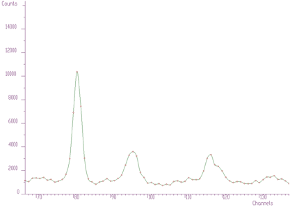
Example of the original spectrum and estimated background (INCREASING CLIPPING WINDOW)
** E-mail : morhac@savba.sk **
This function calculates background spectrum from source spectrum. The result is placed in the vector pointed by spectrum pointer. On successful completion it returns 0. On error it returns pointer to the string describing error.
char *Background1(float *spectrum,
                  int size,
                  int number_of_iterations);
Function parameters:
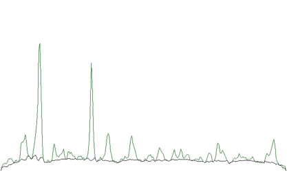
spectrum pointer to the vector of source spectrumsize length of spectrumnumber_of_iterations or width of the clipping windowThe function allows to separate useless spectrum information (continuous background) from peaks, based on Sensitive Nonlinear Iterative Peak Clipping Algorithm. In fact it represents second order difference filter (-1,2,-1). The basic algorithm is described in detail in [1], [2].
\[ v_p(i)= min\left\{v_{p-1} , \frac{[v_{p-1}(i+p)+v_{p-1}(i-p)]}{2} \right\} \]
where p can be changed
from 1 up to a given parameter value w by incrementing it in each iteration step by 1-INCREASING CLIPPING WINDOW
from a given value w by decrementing it in each iteration step by 1- DECREASING CLIPPING WINDOW
An example of the original spectrum and estimated background (INCREASING CLIPPING WINDOW) is given in the Figure 1.1 .
Example of the original spectrum and estimated background (INCREASING CLIPPING WINDOW)
One can notice that on the edges of the peaks the estimated background goes under the peaks. An alternative approach is to decrease the clipping window from a given value to the value of one (DECREASING CLIPPING WINDOW). Then the result obtained is given in the Figure 1.2.
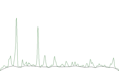
An alternative approach is to decrease the clipping window from a given value to the value of one (DECREASING CLIPPING WINDOW)
The estimated background is smoother. The method does not deform the shape of peaks.
However sometimes the shape of the background is very complicated. The second order filter is insufficient. Let us illustrate such a case in the Figure 1.3. The forth order background estimation filter gives better estimate of complicated background (the clipping window w=10).
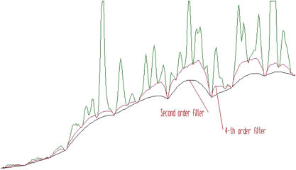
The forth order background estimation filter gives better estimate of complicated background
4-th order algorithm ignores linear as well as cubic component of the background. In this case the filter is (1,-4,6,-4,1). In general the allowed values for the order of the filter are 2, 4, 6, 8. An example of the same spectrum estimated with the clipping window w=40 and with filters of the orders 2, 4, 6, 8 is given in the Figure 1.4.
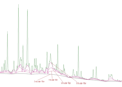
The same spectrum estimated with the clipping window w=40 and with filters of the orders 2, 4, 6, 8
Sometimes it is necessary to include also the Compton edges into the estimate of the background. In Figure 1.5 we present the example of the synthetic spectrum with Compton edges. The background was estimated using the 8-th order filter with the estimation of the Compton edges and decreasing clipping window. In the lower part of the Figure we present the background, which was added to the synthetic spectrum. One can observe good coincidence with the estimated background. The method of the estimation of Compton edge is described in detail in [3].
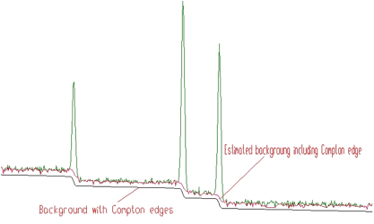
Synthetic spectrum with Compton edges
The generalized form of the algorithm is implemented in the function.
char *Background1General(float *spectrum,
                         int size,
                         int number_of_iterations,
                         int direction,
                         int filter_order,
                         bool compton);
The meaning of the parameters is as follows:
spectrum pointer to the vector of source spectrumsize length of spectrum vectornumber_of_iterations maximal width of clipping window,direction direction of change of clipping window. Possible values:
filter_order order of clipping filter. Possible values:
compton logical variable whether the estimation of Compton edge will be included. Possible values:
This basic background estimation function allows to separate useless spectrum information (2D-continuous background and coincidences of peaks with background in both dimensions) from peaks. It calculates background spectrum from source spectrum. The result is placed in the array pointed by spectrum pointer. On successful completion it returns 0. On error it returns pointer to the string describing error.
char *Background2(float **spectrum,
                  int sizex,
                  int sizey,
                  int number_of_iterations);
Function parameters:
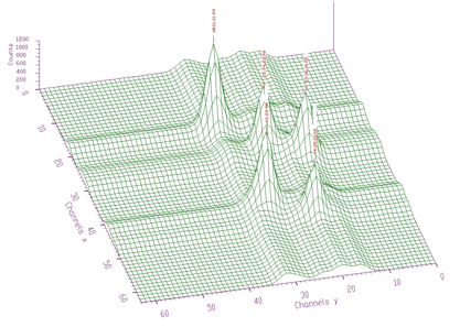
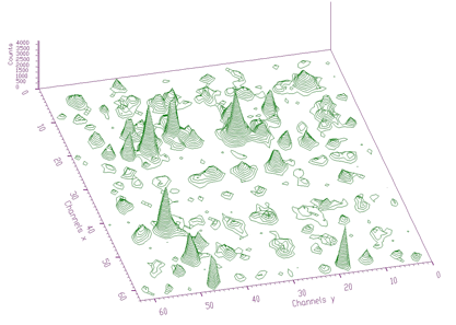
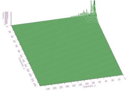
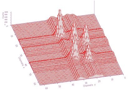
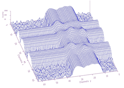
spectrum pointer to the array of source spectrumsizex x length of spectrumsizey y length of spectrumnumber_of_iterations width of the clipping windowIn Figure 1.6 we present an example of 2-dimensional spectrum before background elimination.
2-dimensional spectrum before background elimination
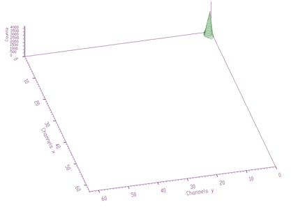
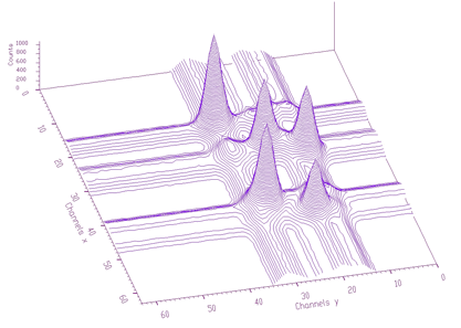
Estimated background is shown in Figure 1.7. After subtraction we get pure 2-dimensional peaks.
Estimated background
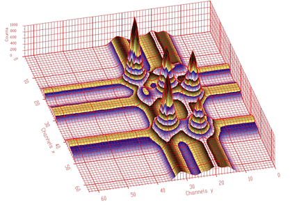
Analogously to 1-dimensional case we have generalized also the function for 2-dimensional background estimation. Sometimes the width of peaks in both dimensions are different. As an example we can introduce n-gamma 2-dimensional spectra. Then it is necessary to set different widths of clipping window in both dimensions. In Figure 1.8 we give an example of such a spectrum.
It is necessary to set different widths of clipping window in both dimensions
Spectrum after background estimation (clipping window 10 for x-direction, 20 for y- direction) and subtraction is given in Figure 1.9.
Spectrum after background estimation (clipping window 10 for x-direction, 20 for y- direction) and subtraction
Background estimation can be carried out using the algorithm of successive comparisons [1] or .based on one-step filtering algorithm given by formula:
\[ v_{p}(i) = min\left\{v_{p-1}(i) , \frac{ \left[\begin{array}{c} -v_{p-1}(i+p,j+p)+2*v_{p-1}(i+p,j)-v_{p-1}(i+p,j-p) \\ +2*v_{p-1}(i,j+p)+2*v_{p-1}(i,j-p) \\ -v_{p-1}(i-p,j+p)+2*v_{p-1}(i-p,j)-v_{p-1}(i-p,j-p) \end{array}\right] }{4} \right\} \]
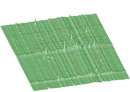
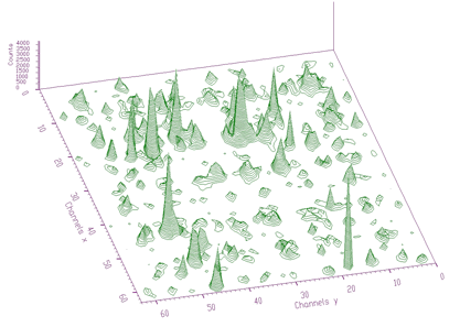
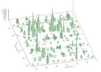
Illustrating example is given in the following 3 Figures. In Figure 1.10 we present original (synthetic) 2-dimensional spectrum. In the Figure 1.11. we have spectrum after background elimination using successive comparisons algorithm and in Figure 1.12 after elimination using one-step filtering algorithm.
Original (synthetic) 2-dimensional spectrum
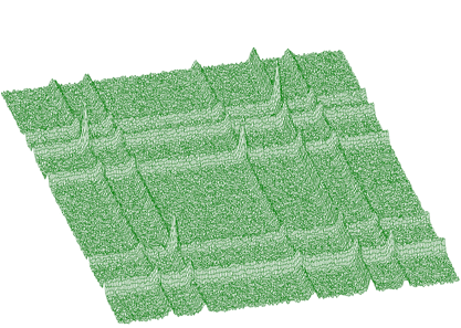
Spectrum after background elimination using successive comparisons algorithm
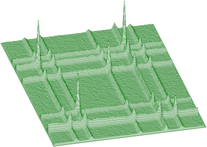
Spectrum after elimination using one-step filtering algorithm
One can notice artificial ridges in the spectrum in Figure 1.11. In the estimation using filtration algorithm this effect disappears. The general function for estimation of 2-dimensional background with rectangular ridges has the form
char *Background2RectangularRidges(float **spectrum,
                                   int sizex,
                                   int sizey,
                                   int number_of_iterations_x,
                                   int number_of_iterations_y,
                                   int direction,
                                   int filter_order,
                                   int filter_type);
This function calculates background spectrum from source spectrum. The result is placed to the array pointed by spectrum pointer.
Function parameters:
spectrum pointer to the array of source spectrumsizex x length of spectrumsizey y length of spectrumnumber_of_iterations_x-maximal x width of clipping windownumber_of_iterations_y-maximal y width of clipping windowdirection direction of change of clipping window. Possible values:
filter_order-order of clipping filter. Possible values:
filter_type determines the algorithm of the filtering. Possible values:
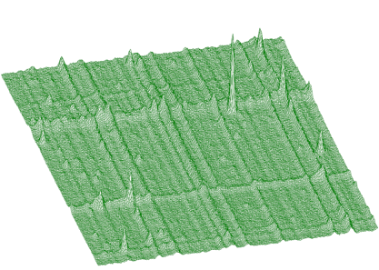
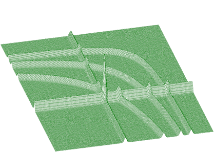
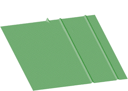
In what follows we describe a function to estimate continuous 2-dimensional background together with rectangular and skew ridges. In Figure 1.13 we present a spectrum of this type.
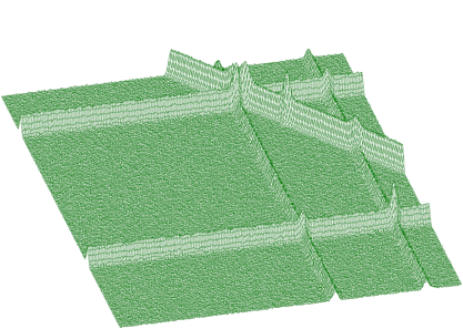
Function to estimate continuous 2-dimensional background together with rectangular and skew ridges
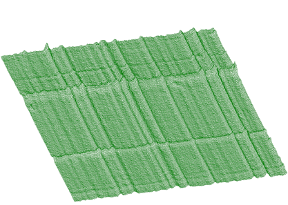
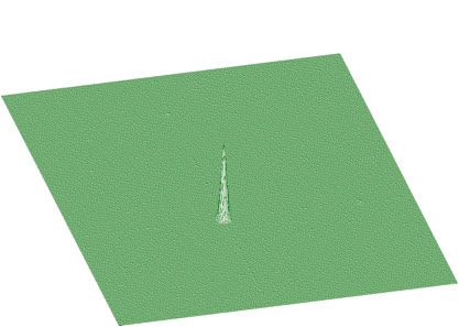
The goal is to remove rectangular as well as skew ridges from the spectrum and to leave only 2-dimensional coincidence peaks. After applying background elimination function and subtraction we get the two dimensional peaks presented in Figure 1.14
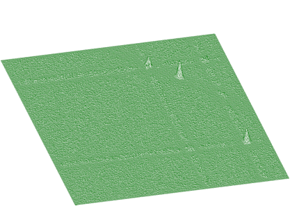
Two dimensional peaks obtained after applying background elimination function and subtraction
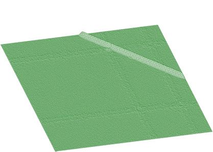
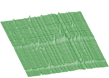
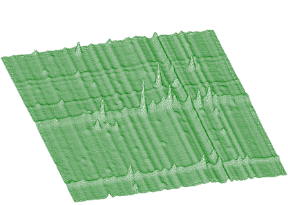
In Figures 1.15 and 1.16 we present experimental spectrum with skew ridges and estimated background, respectively.
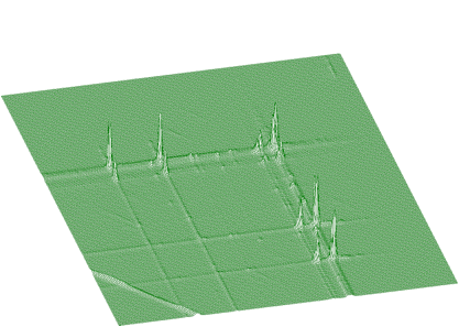
Experimental spectrum with skew ridges
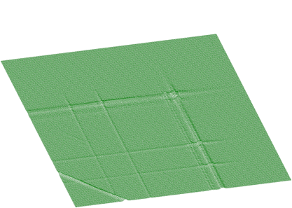
Experimental spectrum with estimated background
The function for the estimation of background together with skew ridges has the form
char *Background2SkewRidges(float **spectrum,
                            int sizex,
                            int sizey,
                            int number_of_iterations_x,
                            int number_of_iterations_y,
                            int direction,
                            int filter_order);
The result is placed to the array pointed by spectrum pointer.
Function parameters:
spectrum pointer to the array of source spectrumsizex x length of spectrumsizey y length of spectrumnumber_of_iterations_x maximal x width of clipping windownumber_of_iterations_y maximal y width of clipping windowdirection direction of change of clipping window. Possible values:
filter_order order of clipping filter. Possible values:
Next we present the function that estimates the continuous background together with rectangular, and nonlinear ridges. To illustrate the data of such a form we present synthetic data shown in Figure 1.17. The estimated background is given in Figure 1.18. Pure Gaussian after subtracting the background from the original spectrum is shown in Figure 1.19
Synthetic data

Estimated background
Pure Gaussian after subtracting the background from the original spectrum
The function to estimate also the nonlinear ridges has the form
char *Background2NonlinearRidges(float **spectrum,
                                 int sizex,
                                 int sizey,
                                 int number-of-iterations-x,
                                 int number-of-iterations-y,
                                 int direction,
                                 int filter_order);
The result is placed to the array pointed by spectrum pointer..
Function parameters:
spectrum pointer to the array of source spectrumsizex x length of spectrumsizey y length of spectrumnumber_of_iterations_x maximal x width of clipping windownumber_of_iterations_y maximal y width of clipping windowdirection direction of change of clipping window. Possible values:
filter_order order of clipping filter. Possible values:
The information contained in the skew ridges and non-linear ridges can be interesting and one may wish to separate it from the rectangular ridges. Therefore we have implemented also two functions allowing to estimate ridges only in the direction rectangular to x- axis and y-axis. Let us have both rectangular and skew ridges from spectrum given in Figure 1.13 estimated using above described function Background2SkewRidges(Figure 1.20).
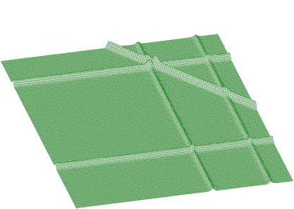
Background2SkewRidges9
Now let us estimate ridges rectangular to x-axis and y-axis (Figures 1.21, 1.22)
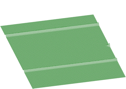
Ridges rectangular to x-axis
ridges rectangular to y-axis
After subtraction these data from spectrum in Figure 1.20, we get separated skew ridge given in Figure 1.23.
Separated skew ridge
The functions for estimation of 1-dimensional ridges in 2-dimensional spectra have the forms
char *Background2RectangularRidgesX(float **spectrum,
                                    int sizex,
                                    int sizey,
                                    int number-of-iterations,
                                    int direction,
                                    int filter_order);
Function parameters:
spectrum pointer to the array of source spectrumsizex x length of spectrumsizey y length of spectrumnumber_of_iterations maximal x width of clipping windowdirection direction of change of clipping window. Possible values:
filter_order order of clipping filter. Possible values:
char *Background2RectangularRidgesY(float **spectrum,
                                    int sizex,
                                    int sizey,
                                    int number_of_iterations,
                                    int direction,
                                    int filter_order);
Function parameters:
spectrum pointer to the array of source spectrumsizex x length of spectrumsizey y length of spectrumnumber_of_iterations maximal width of clipping windowdirection direction of change of clipping window. Possible values:
filter_order order of clipping filter. Possible values
-1-DIMENSIONAL SPECTRA
The operation of the smoothing is based on the convolution of the original data with the filter of the type
(1,2,1)/4 -three points smoothing
(-3,12,17,12,-3)/35 -five points smoothing
(-2,3,6,7,6,3,-2)/21 -seven points smoothing
(-21,14,39,54,59,54,39,14,-21)/231 -nine points smoothing
(-36,9,44,69,84,89,84,69,44,9,-36)/429 -11 points smoothing
(-11,0,9,16,21,24,25,24,21,16,9,0,-11)/143 -13 points smoothing
(-78,-13,42,87,122,147,162,167,162,147,122,87,42,-13,-78)/1105 -15 points smoothing. The function for one-dimensional smoothing has the form
char *Smooth1(float *spectrum,
              int size,
              int points);
This function calculates smoothed spectrum from source spectrum. The result is placed in the vector pointed by spectrum pointer.
Function parameters:
spectrum pointer to the vector of source spectrumsize length of spectrumpoints width of smoothing window. Allowed values
An example of 1-dimensional spectra smoothing and the influence of the filter width on the data is presented in Figure 2.1
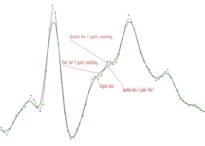
1-dimensional spectra smoothing and the influence of the filter width on the data
The smoothing of the two dimensional data is analogous to the one dimensional case. The width of filter can be chosen independently for each dimension. The form of the 2-D smoothing function is as follows
char *Smooth2(float **spectrum,
              int sizex,
              int sizey,
              int pointsx,
              int pointsy);
This function calculates smoothed spectrum from source spectrum. The result is placed in the array pointed by spectrum pointer.
Function parameters:
spectrum pointer to the array of source spectrumsizex x length of spectrumsizey y length of spectrumpointsx,pointsy width of smoothing window. Allowed values:
An example of 2-D original data and data after smoothing is given in Figures 2.2, 2.3.
2-D original data
Data after smoothing
The basic function of the 1-dimensional peak searching is in detail described in [4], [5]. It allows to identify automatically the peaks in a spectrum with the presence of the continuous background and statistical fluctuations - noise. The algorithm is based on smoothed second differences that are compared to its standard deviations. Therefore it is necessary to pass a parameter of sigma to the peak searching function. The algorithm is selective to the peaks with the given sigma. The form of the basic peak searching function is
Int-t Search1(const float *spectrum,
              int size,
              double sigma);
This function searches for peaks in source spectrum. The number of found peaks and their positions are written into structure pointed by one_dim_peak structure pointer.
Function parameters:
source pointer to the vector of source spectrump pointer to the one_dim_peak structure pointersize length of source spectrumsigma sigma of searched peaksThe structure one_dim_peak has the form:
struct one_dim_peak{
int number_of_peaks;
double position[MAX_NUMBER_OF_PEAKS1];
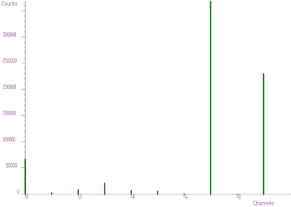
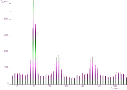
};An example of simple one-dimensional spectrum with identified peaks is given in Figure 3.1.
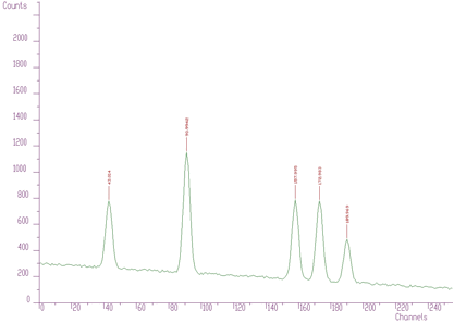
Simple one-dimensional spectrum with identified peaks
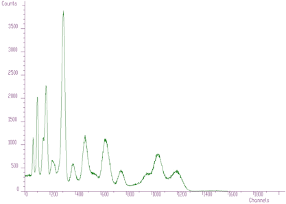
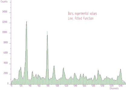
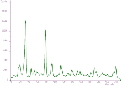
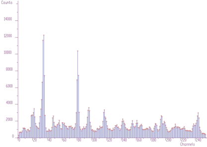
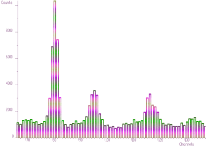
An example of 1-dimensional experimental spectrum with many identified peaks is given in Figure 3.2.
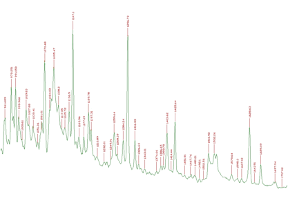
1-dimensional experimental spectrum with many identified peaks
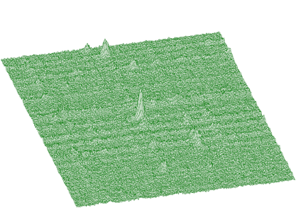
However when we have noisy data the number of peaks can be enormous. One such an example is given in Figure 3.3. Therefore it can be useful to have possibility to set a threshold value and to consider only the peaks higher than this threshold (see Figure 3.4, only three peaks were identified, threshold=50.) The value in the center of the peak value[i] minus the average value in two symmetrically positioned channels (channels i-3*sigma, i+3*sigma) must be greater than threshold. Otherwise the peak is ignored.
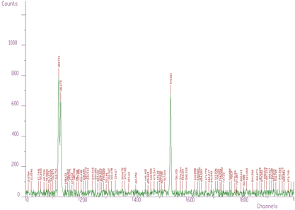
With noisy data the number of peaks can be enormous
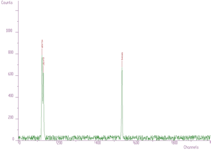
Iwth threshold=50, only three peaks were identified
An alternative approach was proposed in [6].. The algorithm generates new invariant spectrum based on discrete Markov chains. In this spectrum the noise is suppressed, the spectrum is smoother than the original one. On the other hand it emphasizes peaks (depending on the averaging window). The example of the part of original noisy spectrum and Markov spectrum for window=3 is given in Figure 3.5 Then the peaks can found in Markov spectrum using standard above presented algorithm.
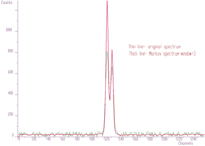
Part of original noisy spectrum and Markov spectrum for window=3
The form of the generalized peak searching function is as follows.
Int-t Search1General(float *spectrum,
                     int size,
                     float sigma,
                     int threshold,
                     bool markov,
                     int aver-window);
This function searches for peaks in source spectrum. The number of found peaks and their positions are written into structure pointed by one_dim_peak structure pointer.
Function parameters:
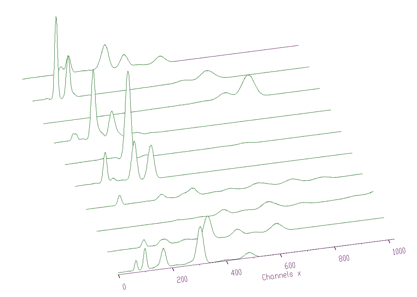
spectrum pointer to the vector of source spectrum source spectrum is replaced by new spectrum calculated using Markov chains method.size length of source spectrumsigma sigma of searched peaksthreshold threshold value for selecting of peaksmarkov logical variable, if it is true, first the source spectrum is replaced by new spectrum calculated using Markov chains method.aver_window averaging window used in calculation of Markov spectrum, applies only for markov variable is trueThe methods of peak searching are sensitive to the sigma. Usually the sigma value is known beforehand. It also changes only slightly with the energy. We have investigated as well the robustness of the proposed algorithms to the spectrum with the peaks with sigma changing from 1 to 10 (see Figure 3.6).
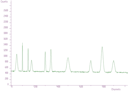
Robustness of the proposed algorithms to the spectrum with the peaks with sigma changing from 1 to 10
We applied peak searching algorithm based on Markov approach. We changed sigma in the interval from 1 to 10. The spectra for averaging windows 3, 5, 10 are shown in Figure 3.7.
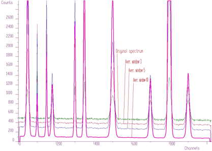
Spectra for averaging windows 3, 5, 10
When we applied peak searching function to the Markov spectrum averaged with the window=10, we obtained correct estimate of all 10 peak positions for sigma=2,3,4,5,6,7,8. It was not the case when we made the same experiment with the original spectrum. For all sigmas some peaks were not discovered.
The basic function of the 2-dimensional peak searching is in detail described in [4].. It identifies automatically the peaks in a spectrum with the presence of the continuous background, statistical fluctuations as well as coincidences of background in one dimension and peak in the other one-ridges. The form of the basic function of 2-dimensional peak searching is
Int-t Search2(const float **source,
              int sizex,
              int sizey,
              double sigma);
This function searches for peaks in source spectrum .The number of found peaks and their positions are written into structure pointed by two_dim_peak structure pointer.
Function parameters:
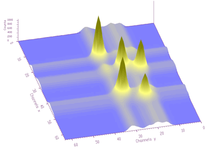
source pointer to the vector of source spectrumsizex x length of source spectrumsizey y length of source spectrumsigma sigma of searched peaksAn example of the two-dimensional spectrum with the identified peaks is shown in Figure 3.8.
Two-dimensional spectrum with the identified peaks
We have also generalized the peak searching function analogously to one dimensional data. The generalized peak searching function for two dimensional spectra has the form
Int-t Search2General(float **source,
                     int sizex,
                     int sizey,
                     double sigma,
                     int threshold,
                     bool markov,
                     int aver-window);
This function searches for peaks in source spectrum. The number of found peaks and their positions are written into structure pointed by two_dim_peak structure pointer.
Function parameters:
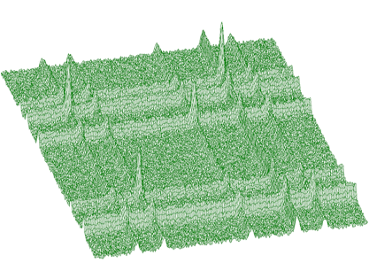
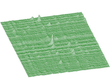
source pointer to the vector of source spectrumsizex x length of source spectrumsizey y length of source spectrumsigma sigma of searched peaksthreshold threshold value for selection of peaksmarkov logical variable, if it is true, first the source spectrum is replaced by new spectrum calculated using Markov chains method.aver_window averaging window of searched peaks (applies only for Markov method)An example of experimental 2-dimensional spectrum is given in Figure 3.9. The number of peaks identified by the function now is 295.
Experimental 2-dimensional spectrum
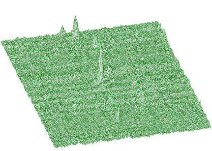
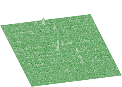
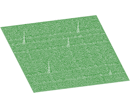
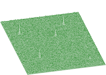
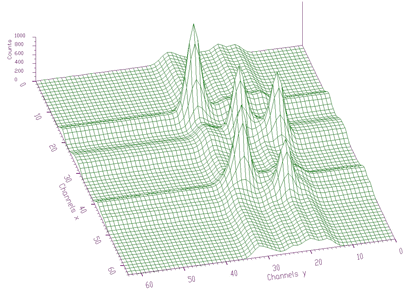
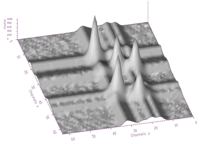
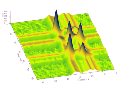
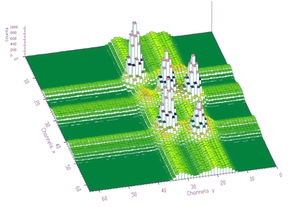
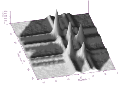
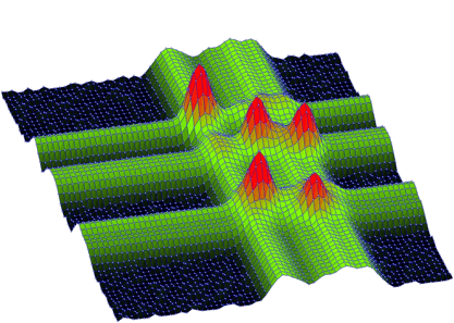
The function works even for very noisy data. In Figure 3.10 we present synthetic 2-dimensional spectrum with 5 peaks. The method should recognize what is real 2-dimensional peak and what is the crossing of two 1-dimensional ridges The Markov spectrum with averaging window=3 is given in Figure 3.11. One can observe that this spectrum is smoother than the original one. After applying the general peak searching function to the Markov spectrum with sigma=2, and threshold=600, we get correctly identified peaks.
Synthetic 2-dimensional spectrum with 5 peaks
Markov spectrum with averaging window=3
Mathematical formulation of the convolution system is:
\[ y(i) = \sum_{k=0}^{N-1}h(i-k)x(k), i=0,1,2,...,N-1 \]
where h(i) is the impulse response function, x, y are input and output vectors,
respectively, N is the length of x and h vectors. In matrix form we have:
\[ \left[\begin{array}{c} y(0)\\ y(1)\\ .\\ .\\ .\\ .\\ .\\ y(2N-2)\\ y(2N-1) \end{array}\right] = \left[\begin{array}{cccccc} h(0) & 0 & 0 & 0 & ... & 0\\ h(1) & h(0) & 0 & 0 & ... & 0\\ . & h(1) & h(0) & 0 & ... & 0\\ h(N-1) & . & h(1) & h(0) & ... & 0\\ 0 & h(N-1) & . & h(1) & ... & 0\\ 0 & 0 & h(N-1) & . & ... & h(0)\\ 0 & 0 & 0 & h(N-1) & ... & h(1)\\ . & . & . & . & ... & .\\ 0 & 0 & 0 & 0 & ... & h(N-1) \end{array}\right] \left[\begin{array}{c} x(0)\\ x(1)\\ x(2)\\ .\\ .\\ y(N-1) \end{array}\right] \]
Let us assume that we know the response and the output vector (spectrum) of the above given system. The deconvolution represents solution of the overdetermined system of linear equations, i.e., the calculation of the vector x.
The goal of the deconvolution methods is to improve the resolution in the spectrum and to decompose multiplets. From mathematical point of view the operation of deconvolution is extremely critical as well as time consuming operation. From all the methods studied the Gold deconvolution (decomposition) proved to work as the best one. It is suitable to process positive definite data (e.g. histograms). In detail the method is described in [7], [8].
\[ y = Hx \] \[ H^T=H^THx \] \[ y^{'} = H^{'}x \] \[x_{i}^{(k+1)}=\frac{y_{i}^{'}}{\sum_{m=0}^{N-1}H_{im}^{'}x_{m}^{(k)}}x_{i}^{(k)}, i=0,1,...,N-1, \] where: \[ k=1,2,3,...,I \] \[ x^{(0)} = [1,1,...,1]^T \]
The basic function has the form
char *Deconvolution1(float *source,
                     const float *resp,
                     int size,
                     int number-of-iterations);
This function calculates deconvolution from source spectrum according to response spectrum.
Function parameters:
source pointer to the vector of source spectrumresp pointer to the vector of response spectrumsize length of source and response spectranumber_of_iterations for details see [8]As an illustration of the method let us introduce small example. In Figure 4.1 we present original 1-dimensional spectrum. It contains multiplets that cannot be directly analyzed. The response function (one peak) is given in Figure 4.2. We assume the same response function (not changing the shape) along the entire energy scale. So the response matrix is composed of mutually shifted response functions by one channel, however of the same shape.
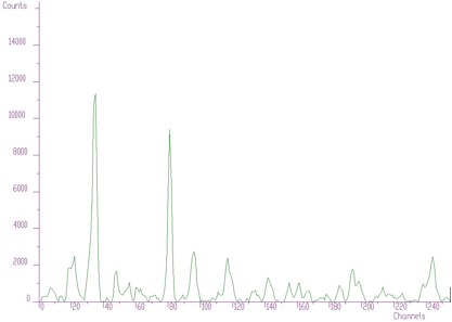
Original 1-dimensional spectrum
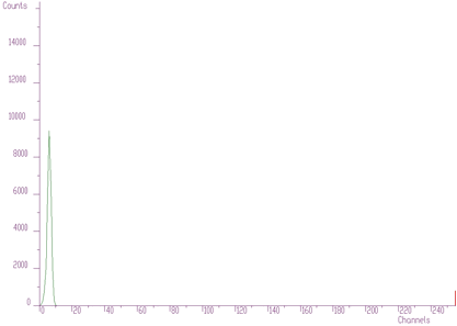
Response function (one peak)
The result after deconvolution is given in Figure 4.3. It substantially improves the resolution in the spectrum.
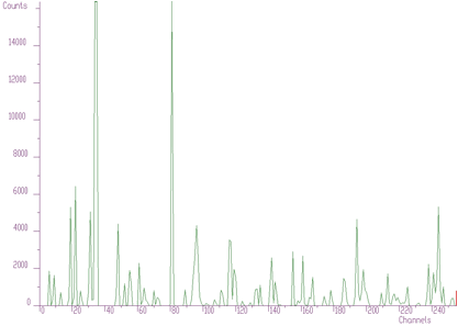
Result after deconvolution
We have developed a new high resolution deconvolution algorithm. We have observed that the Gold deconvolution converges to its stable state (solution). It is useless to increase the number of iterations, the result obtained does not change. To continue in decreasing the width of peaks we have found that when the solution reaches its stable state it is necessary to stop iterations, then to change the vector in a way and repeat again the Gold deconvolution . We have found that to change the particular solution we need to apply non-linear boosting function to it. The power function proved to give the best results. At the beginning the function calculates exact solution of the Toeplitz system of linear equations.
\[ x^{(0)} = [x_e^2(0),x_e^2(1),...,x_e^2(N-1),]^T\] where : \[ x_e=H^{'-1}y^{'}\] Then it applies the Gold deconvolution algorithm to the solution and carries out preset number of iterations. Then the power function with the exponent equal to the boosting coefficient is applied to the deconvolved data. These data are then used as initial estimate of the solution of linear system of equations and again the Gold algorithm is employed. The whole procedure is repeated number_of_repetitions times.
The form of the high-resolution deconvolution function is
char *Deconvolution1HighResolution(float *source,
                                   const float *resp,
                                   int size,
                                   int number-of-iterations,
                                   int number-of-repetitions,
                                   double boost);
This function calculates deconvolution from source spectrum according to response spectrum
The result is placed in the vector pointed by source pointer.
Function parameters:
source pointer to the vector of source spectrumresp pointer to the vector of response spectrumsize length of source and response spectranumber_of_iterations for details we refer to manualnumber_of_repetitions for details we refer to manualboost boosting factor, for details we refer to manualThe result obtained using the data from Figures 4.1, 4.2 and applying the high resolution deconvolution is given in Figure 4.4. It decomposes the peaks even more (practically to 1, 2 channels).
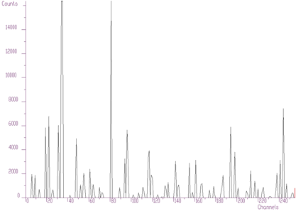
Result obtained using the data from Figures 4.1, 4.2 and applying the high resolution deconvolution
Another example of synthetic data is given in Figure 4.5. We have positioned the two peaks very close to each other (2 channels). The method of high resolution deconvolution has decomposed these peaks practically to one channel. The original data are shown as polyline, the data after deconvolution as bars. The numbers at the bars denote the heights of bars and the numbers in parenthesis the original area of peaks. The area of original peaks is concentrated into one channel.
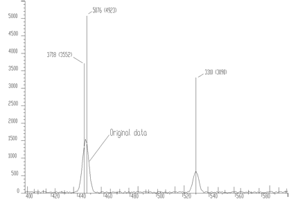
Example of synthetic data
Up to now we assumed that the shape of the response is not changing. However the method of Gold decomposition can be utilized also for the decomposition of input data (unfolding) with completely different responses. The form of the unfolding function is as follows
char *Deconvolution1Unfolding(float *source,
                              const float **resp,
                              int sizex,
                              int sizey,
                              int number-of-iterations);
This function unfolds source spectrum according to response matrix columns. The result is placed in the vector pointed by source pointer.
Function parameters:
source pointer to the vector of source spectrumresp pointer to the matrix of response spectrasizex length of source spectrum and # of rows of response matrixsizey # of columns of response matrixnumber_of_iterationsNote!!! sizex must be >= sizey. After decomposition the resulting channels are written back to the first sizey channels of the source spectrum.
The example of the response matrix composed of the responses of different chemical elements is given in Figure 4.6
Example of the response matrix composed of the responses of different chemical elements
The original spectrum before unfolding is given in Figure 4.7. The obtained coefficients after unfolding, i.e., the contents of the responses in the original spectrum is presented in the Figure 4.8.
Original spectrum before unfolding
Contents of the responses in the original spectrum
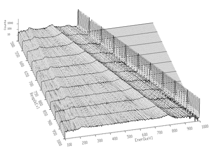
Another example where we have used unfolding method is the decomposition of continuum of gamma-ray spectra. Using simulation and interpolation techniques we have synthesized the response matrix (size 3400x3400 channels) of Gammasphere spectrometer (Figure 4.9). Its detail is presented in Figure 4.10. The original spectrum of Co56 before and after continuum decomposition are presented in Figures 4.11, 4.12, respectively.
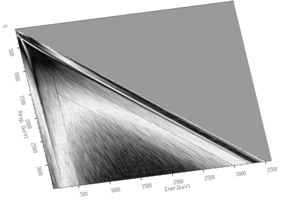
Response matrix (size 3400x3400 channels) of Gammasphere spectrometer
Detail of Figure 4.9
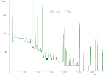
Original spectrum of Co56 before continuum decomposition
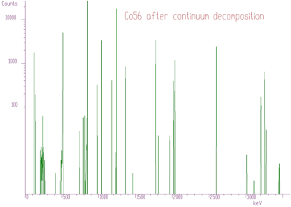
Original spectrum of Co56 after continuum decomposition
We have extended the method of Gold deconvolution also for 2-dimensional data. Again the goal of the deconvolution methods is to improve the resolution in the spectrum and to decompose multiplets. In detail the method of optimized 2-dimensional deconvolution is described in [8].
Mathematical formulation of 2-dimensional convolution system is as follows
\[ y(i_1,i_2) = \sum_{k_1=0}^{N_1-1}\sum_{k_2=0}^{N_2-1}h(i_1-k_1,i_2-k_2)x(k_1,k_2), i_1=0,1,2,...,N_1-1, i_2=0,1,2,...,N_2-1 \]
Assuming we know the output spectrum y and the response spectrum h,the task is to calculate the matrix x.
The basic function has the form
char *Deconvolution2(float **source,
                     const float **resp,
                     int sizex,
                     int sizey,
                     int niter);
This function calculates deconvolution from source spectrum according to response spectrum. The result is placed in the matrix pointed by source pointer.
Function parameters:
source pointer to the matrix of source spectrumresp pointer to the matrix of response spectrumsizex x length of source and response spectrasizey y length of source and response spectranumber_of_iterations for details see [8]The example of 2-dimensional spectrum before deconvolution is presented in Figure 4.13. In the process of deconvolution we have used the response matrix (one peak shifted to the beginning of the coordinate system) given in Figure 4.14. Employing the Gold deconvolution algorithm implemented in the decon2 function we get the result shown in Figure 4.15. One can notice that the peaks became narrower thus improving the resolution in the spectrum.
2-dimensional spectrum before deconvolution
Response matrix (one peak shifted to the beginning of the coordinate system)
Result obtained employing the Gold deconvolution algorithm implemented in the decon2 function
Analogously to 1-dimensional case we have developed high-resolution 2-dimensional deconvolution. From the beginning the exact solution of the cyclic convolution 2-dimensional system is calculated. Then we apply the repeated deconvolution with boosting in the same way like in 1- dimensional case. The form of the high-resolution 2-dimensional deconvolution function is:
char *Deconvolution2HighResolution(float **source,
                                   const float **resp,
                                   int sizex,
                                   int sizey,
                                   int number_of_iterations,
                                   int number_of_repetitions,
                                   double boost);
This function calculates deconvolution from source spectrum
according to response spectrum
The result is placed in the matrix pointed by source pointer.
Function parameters:
source pointer to the matrix of source spectrumresp pointer to the matrix of response spectrumsizex x length of source and response spectrasizey y length of source and response spectranumber_of_iterationsnumber_of_repetitionsboost boosting factorWhen we apply this function to the data from Figure 4.13 using response matrix given in Figure 4.14 we get the result shown in Figure 4.16. It is apparent that the high-resolution deconvolution decomposes the input data even more than the original Gold deconvolution.
Result obtained applying Deconvolution2HighResolution to the data from Figure 4.13 using response matrix given in Figure 4.14
A lot of algorithms have been developed (Gauss-Newton, Levenber-Marquart conjugate gradients, etc.) and more or less successfully implemented into programs for analysis of complex spectra. They are based on matrix inversion that can impose appreciable convergence difficulties mainly for large number of fitted parameters. Peaks can be fitted separately, each peak (or multiplets) in a region or together all peaks in a spectrum. To fit separately each peak one needs to determine the fitted region. However it can happen that the regions of neighboring peaks are overlapping (mainly in 2-dimensional spectra). Then the results of fitting are very poor. On the other hand, when fitting together all peaks found in a spectrum, one needs to have a method that is stable (converges) and fast enough to carry out fitting in reasonable time. The gradient methods based on the inversion of large matrices are not applicable because of two reasons
calculation of inverse matrix is extremely time consuming;
due to accumulation of truncation and rounding-off errors the result can become worthless.
We have implemented two kinds of fitting functions. The first approach is based on the algorithm without matrix inversion [9]-awmi algorithm. It allows to fit large blocks of data and large number of parameters.
The other one is based on calculation of the system of linear equations using Stiefel-Hestens method [10]. It converges faster than awmi algorithm, however it is not suitable to fit large number of parameters.
\[ \chi^2 = \frac{1}{N-M}\sum_{i=1}^{N}\frac{[y_i-f(i,a)]^2}{y_i} \]
where \(i\) is the channel in the fitted spectrum, \(N\) is the number of channels in the fitting subregion, \(M\) is the number of free parameters, \(y_i\) is the content of the i-th channel, \(a\) is a vector of the parameters being fitted and \(f(i,a)\) is a fitting or peak shape function.
Instead of the weighting coefficient \(y_i\) in the denominator of the above given formula one can use also the value of \(f(i,a)\). It is suitable for data with poorstatistics [11], [12].
The third statistic to be optimized, which is implemented in the fitting functions is Maximum Likelihood Method. It is of the choice of the user to select suitable statistic..
\[ \sum_{i=1}^{N} \frac{y_i-f(i,a^{(t)})}{y_i} \frac{\partial f(i,a^t)}{\partial a_k}= \sum_{j=1}^{M}\sum_{i=1}^{N} \frac{\partial f(i,a^{(t)})}{\partial a_j} \frac{\partial f(i,a^{(t)})}{\partial a_k} \Delta a_j^{(t)} \]
in \(\gamma\)-ray spectra we have to fit together tens, hundreds of peaks simultaneously that represent sometimes thousands of parameters.
the calculation of the inversion matrix of such a size is practically impossible.
the awmi method is based on the assumption that off-diagonal terms in the matrix A are equal to zero.
\[ \Delta a_{k}^{(t+1)} = \alpha^{(t)} \frac{ \sum_{i=1}^{N} \frac{e_{i}^{(t)}}{y_i}\frac{\partial f(i,a^{(t)})}{\partial a_k} }{ \sum_{i=1}^{N} \left[ \frac{\partial f(i,a^{(t)})}{\partial a_k}\right]^2\frac{1}{y_i} } \]
where the error in the channel \(i\) is \(e_{i}^{(t)} = y_i-f(i,a^{(t)}); k=1,2,...,M\) and \(\alpha^{(t)}=1\) if the process is convergent or \(\alpha^{(t)}=0.5 \alpha^{(t-1)}\) if it is divergent. Another possibility is to optimize this coefficient.
the error of \(k\)-th parameter estimate is
\[ \Delta a_k^{(e)}= \sqrt{\frac {\sum_{i=1}^{N}\frac{e_i^2}{y_i}} {\sum_{i=1}^{N} \left[ \frac{\partial f(i,a^{(t)})}{\partial a_k}\right]^2\frac{1}{y_i}} } \]
algorithm with higher powers w=1,2,3…
\[ \Delta a_{k,w}^{(t+1)}= \alpha^{(t)} \frac {\sum_{i=1}^{N} \frac{e_i}{y_i}\left[ \frac{\partial f(i,a^{(t)})}{\partial a_k}\right]^{2w-1}} {\sum_{i=1}^{N} \left[ \frac{\partial f(i,a^{(t)})}{\partial a_k}\right]^{2w}\frac{1}{y_i}} \]
we have implemented the nonsymmetrical semiempirical peak shape function.
it contains the symmetrical Gaussian as well as nonsymmetrical terms.
\[ f(i,a) = \sum_{i=1}^{M} A(j) \left\{ exp\left[\frac{-(i-p(j))^2}{2\sigma^2}\right] +\frac{1}{2}T.exp\left[\frac{(i-p(j))}{B\sigma}\right] .erfc\left[\frac{(i-p(j))}{\sigma}+\frac{1}{2B}\right] +\frac{1}{2}S.erfc\left[\frac{(i-p(j))}{\sigma}\right] \right\} \]
where \(T,S\) are relative amplitudes and \(B\) is a slope.
Detailed description of the algorithm is given in [13].
The fitting function implementing the algorithm without matrix inversion has the form
char* Fit1Awmi(float *source,
               TSpectrumOneDimFit *p,
               int size);
This function fits the source spectrum. The calling program should fill in input parameters of the one_dim_fit structure The fitted parameters are written into structure pointed by one_dim_fit structure pointer and fitted data are written into source spectrum.
Function parameters:
source pointer to the vector of source spectrump pointer to the one_dim_fit structure pointersize length of source spectrumThe one_dim_fit structure has the form:
class TSpectrumOneDimFit{

public:

   int number_of_peaks;      // input parameter, should be >0
   int number_of_iterations; // input parameter, should be >0
   int xmin;                 // first fitted channel
   int xmax;                 // last fitted channel
   double alpha;             // convergence coefficient, input parameter, it should be
                             // positive number and <=1
   double chi;               // here the function returns resulting chi-square
   int statistic_type;       // type of statistics, possible values
                             // FIT1_OPTIM_CHI_COUNTS (chi square statistics with
                             // counts as weighting coefficients),
                             // FIT1_OPTIM_CHI_FUNC_VALUES (chi square statistics
                             // with function values as weighting coefficients)
                             // FIT1_OPTIM_MAX_LIKELIHOOD
   int alpha_optim;          // optimization of convergence coefficients, possible values
                             // FIT1_ALPHA_HALVING,
                             // FIT1_ALPHA_OPTIMAL
   int power;                // possible values FIT1_FIT_POWER2,4,6,8,10,12
   int fit_taylor;           // order of Taylor expansion, possible values
                             // FIT1_TAYLOR_ORDER_FIRST, FIT1_TAYLOR_ORDER_SECOND

   double position_init[MAX_NUMBER_OF_PEAKS1]; // initial values of
                                               // peaks positions, input parameters
   double position_calc[MAX_NUMBER_OF_PEAKS1]; // calculated values
                                               // of fitted positions, output parameters
   double position_err[MAX_NUMBER_OF_PEAKS1];  // position errors
   bool fix_position[MAX_NUMBER_OF_PEAKS1];    // logical vector which allows to fix
                                               // appropriate positions (not fit). However they
                                               // are present in the estimated functional
   double amp_init[MAX_NUMBER_OF_PEAKS1];      // initial values of peaks
                                               // amplitudes, input parameters
   double amp_calc[MAX_NUMBER_OF_PEAKS1];      // calculated values of
                                               // fitted amplitudes, output parameters
   double amp_err[MAX_NUMBER_OF_PEAKS1];       // amplitude errors
   bool fix_amp[MAX_NUMBER_OF_PEAKS1]i;        // logical vector, which allows to fix
                                               // appropriate amplitudes (not fit). However they
                                               // are present in the estimated functional
   double area[MAX_NUMBER_OF_PEAKS1];          // calculated areas of peaks
   double area_err[MAX_NUMBER_OF_PEAKS1];      // errors of peak areas

   double sigma_init // sigma parameter, see peak shape function
   double sigma_calc;
   double sigma_err;
   bool fix_sigma;
   double t_init     // t parameter, , see peak shape function
   double t_calc;
   double t_err;
   bool fix_t;
   double b_init     // b parameter, , see peak shape function
   double b_calc;
   double b_err;
   bool fix_b;
   double s_init;    // s parameter, , see peak shape function
   double s_calc;
   double s_err;
   bool fix_s;
   double a0_init;   // backgroud is estimated as a0+a1*x+a2*x*x
   double a0_calc;
   double a0_err;
   bool fix_a0;
   double a1_init;
   double a1_calc;
   double a1_err;
   bool fix_a1;
   double a2_init;
   double a2_calc;
   double a2_err;
   bool fix_a2;
 };
As an example we present simple 1-dimensional synthetic spectrum with 5 peaks. The fit obtained using above given awmi fitting function is given in Figure 5.1. The chi-square achieved in this fit was 0.76873. The input value of the fit (positions of peaks and their amplitudes) were estimated using peak searching function.
Fit obtained using above given awmi fitting function
Let us go to more complicated fit with lot of overlapping peaks Figure 5.2. The initial positions of peaks were determined from original data, using peak searching function. The fit is not very good, as there are some peaks missing.
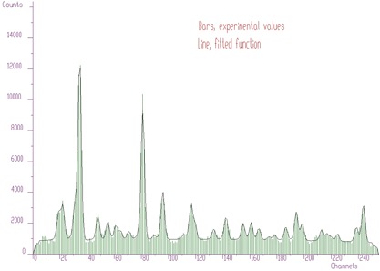
More complicated fit with lot of overlapping peaks
However to analyze the spectrum we can proceed in completely different way employing the sophisticated functions of background elimination and deconvolution. First let us remove background from the original raw data. We get spectrum given in Figure 5.3.
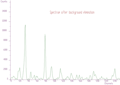
Removed background from the original raw data
Then we can apply the Gold deconvolution function to these data. We obtain result presented in Figure 5.4.
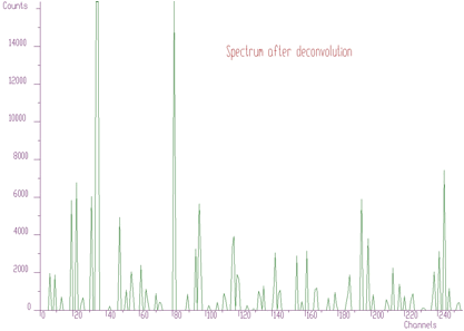
Gold deconvolution function applied to the data
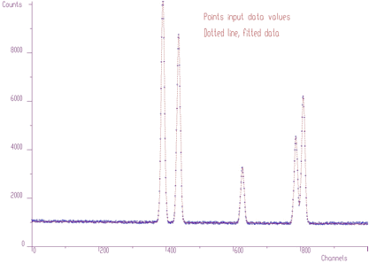
Using peaks searching method, looking just for local maxima, (sigma=0) with appropriate threshold (50), we can estimate initial positions of peaks for fitting function. After the fit of the original experimental spectrum (with background) we obtain the result shown in Figure 5.5. Now the fitted function corresponds much better to experimental values
Fit of the original experimental spectrum (with background)
We have implemented also the fitting function with matrix inversion based on Stiefel-Hestens method of the solution of the system of linear equations. The form of the function is as follows
char *Fit1Stiefel(float *source,
                  TSpectrumOneDimFit* p,
                  int size);
This function fits the source spectrum. The calling program should fill in input parameters of the one_dim_fit structure The fitted parameters are written into structure pointed by one_dim_fit structure pointer and fitted data are written into source spectrum.
Function parameters:
source pointer to the vector of source spectrump pointer to the one_dim_fit structure pointersize length of source spectrumThe structure one_dim_fit is the same as in awmi function. The parameters power, fit_taylor are not applicable for this function
The results for small number of fitted parameters are the same as with awmi function. However it converges faster. The example for data given in Figure 5.1 is given in the following table:
# of iterationsi |
Chi awmi |
Chi-Stiefel |
|
924 |
89.042 |
|
773.15 |
0.96242 |
|
38.13 |
0.77041 |
|
0.90293 |
0.76873 |
|
0.76886 |
0.76873 |
|
0.76873 |
0.76873 |
it is straightforward that for two dimensional spectra one can write
\[ \Delta a_k^{(t+1)}=\alpha^{(t)} \frac {\sum_{i_1=1}^{N_1}\sum_{i_2=1}^{N_2}\frac{e_{i_1,i_2}^{(t)}}{y_{i_1,i_2}} \frac{\partial f(i_1,i_2,a^{(t)})}{\partial a_k}} {\sum_{i_1=1}^{N_1}\sum_{i_2=1}^{N_2} \left[\frac{\partial f(i_1,i_2,a^{(t)})}{\partial a_k} \right]^2 \frac{1}{y_{i_1,i_2}}} \]
analogously for two dimensional peaks we have chosen the peak shape function of the following form
\[ f(i_1,i_2,a) = \sum_{j=1}^{M}\left\{ \begin{array}{l} A_{xy}(j) exp\left\{-\frac{1}{2(1-\rho^2)}\left[ \frac{(i_1-p_x(j))^2}{\sigma_x^2} -\frac{2\rho(i_1-p_x(j))(i_2-p_y(j))}{\sigma_x\sigma_y} +\frac{(i_2-p_y(j))^2}{\sigma_y^2} \right]\right\} \\ +A_x(j) exp\left[-\frac{(i_1-p_{x_1}(j))^2}{2\sigma_x^2} \right] +A_y(j) exp\left[-\frac{(i_2-p_{y_1}(j))^2}{2\sigma_y^2} \right] \end{array} \right\}+b_0+b_1i_1+b_2i_2 \]
The meaning of the parameters is analogous to 1-dimensional case. Again all the details can be found in [13]
The fitting function implementing the algorithm without matrix inversion for 2-dimensional data has the form
char* Fit2Awmi(float **source,
               TSpectrumTwoDimFit* p,
               int sizex,
               int sizey);
This function fits the source spectrum. The calling program should fill in input parameters of the two_dim_fit structure The fitted parameters are written into structure pointed by two_dim_fit structure pointer and fitted data are written back into source spectrum.
Function parameters:
source pointer to the matrix of source spectrump pointer to the two_dim_fit structure pointer, see manualsizex length x of source spectrumsizey length y of source spectrumThe two_dim_fit structure has the form
class TSpectrumTwoDimFit{

public:

   int number_of_peaks;      // input parameter, shoul be>0
   int number_of_iterations; // input parameter, should be >0
   int xmin;                 // first fitted channel in x direction
   int xmax;                 // last fitted channel in x direction
   int ymin;                 // first fitted channel in y direction
   int ymax;                 // last fitted channel in y direction
   double alpha;             // convergence coefficient, input parameter, it should be positive
                             // number and <=1
   double chi;               // here the function returns resulting chi square
   int statistic_type;       // type of statistics, possible values
                             // FIT2_OPTIM_CHI_COUNTS (chi square statistics with
                             // counts as weighting coefficients),
                             // FIT2_OPTIM_CHI_FUNC_VALUES (chi square statistics
                             // with function values as weighting
                             // coefficients),FIT2_OPTIM_MAX_LIKELIHOOD
   int alpha_optim;          // optimization of convergence coefficients, possible values
                             // FIT2_ALPHA_HALVING, FIT2_ALPHA_OPTIMAL
   int power;                // possible values FIT21_FIT_POWER2,4,6,8,10,12
   int fit_taylor;           // order of Taylor expansion, possible values
                             // FIT2_TAYLOR_ORDER_FIRST,
                             // FIT2_TAYLOR_ORDER_SECOND
   double position_init_x[MAX_NUMBER_OF_PEAKS2];  // initial values of x
                                                  // positions of 2D peaks, input parameters
   double position_calc_x[MAX_NUMBER_OF_PEAKS2];  // calculated values
                                                  // of fitted x positions of 2D peaks, output parameters
   double position_err_x[MAX_NUMBER_OF_PEAKS2];   // x position errors of 2D peaks
   bool fix_position_x[MAX_NUMBER_OF_PEAKS2];     // logical vector which allows to fix appropriate
                                                  // x positions of 2D peaks (not fit).
                                                  // However they are present in the estimated functional
   double position_init_y[MAX_NUMBER_OF_PEAKS2];  // initial values of y
                                                  // positions of 2D peaks, input parameters
   double position_calc_y[MAX_NUMBER_OF_PEAKS2];  // calculated values
                                                  // of fitted y positions of 2D peaks, output parameters
   double position_err_y[MAX_NUMBER_OF_PEAKS2];   // y position errors of 2D peaks
   bool fix_position_y[MAX_NUMBER_OF_PEAKS2];     // logical vector which allows to fix appropriate
                                                  // y positions of 2D peaks (not fit).
                                                  // However they are present in the estimated functional
   double position_init_x1[MAX_NUMBER_OF_PEAKS2]; // initial values of x
                                                  // positions of 1D ridges, input parameters
   double position_calc_x1[MAX_NUMBER_OF_PEAKS2]; // calculated values of
                                                  // fitted x positions of 1D ridges, output parameters
   double position_err_x1[MAX_NUMBER_OF_PEAKS2];  // x position errors of 1D ridges
   bool fix_position_x1[MAX_NUMBER_OF_PEAKS2];    // logical vector which allows to fix appropriate
                                                  // x positions of 1D ridges (not fit).
                                                  // However they are present in the estimated functional
   double position_init_y1[MAX_NUMBER_OF_PEAKS2]; // initial values of y
                                                  // positions of 1D ridges, input parameters
   double position_calc_y1[MAX_NUMBER_OF_PEAKS2]; // calculated values
                                                  // of fitted y positions of 1D ridges, output parameters
   double position_err_y1[MAX_NUMBER_OF_PEAKS2];  // y position errors of 1D ridges
   bool fix_position_y1[MAX_NUMBER_OF_PEAKS2];    // logical vector which allows to fix
                                                  // appropriate y positions of 1D ridges (not fit).
                                                  // However they are present in the estimated functional
   double amp_init[MAX_NUMBER_OF_PEAKS2];         // initial values of 2D peaks
                                                  //  amplitudes, input parameters
   double amp_calc[MAX_NUMBER_OF_PEAKS2];         // calculated values of
                                                  // fitted amplitudes of 2D peaks, output parameters
   double amp_err[MAX_NUMBER_OF_PEAKS2];          // amplitude errors of 2D peaks
   bool fix_amp[MAX_NUMBER_OF_PEAKS2];            // logical vector which allows
                                                  // to fix appropriate amplitudes of 2D peaks (not fit).
                                                  // However they are present in the estimated functional
   double amp_init_x1[MAX_NUMBER_OF_PEAKS2];      // initial values of 1D
                                                  // ridges amplitudes, input parameters
   double amp_calc_x1[MAX_NUMBER_OF_PEAKS2];      // calculated values of
                                                  // fitted amplitudes of 1D ridges, output parameters
   double amp_err_x1[MAX_NUMBER_OF_PEAKS2];       // amplitude errors of 1D ridges
   bool fix_amp_x1[MAX_NUMBER_OF_PEAKS2];         // logical vector which alloes to fix
                                                  // appropriate amplitudes of 1D ridges (not fit).
                                                  // However they are present in the estimated functional
   double amp_init_y1[MAX_NUMBER_OF_PEAKS2];      // initial values of 1D
                                                  // ridges amplitudes, input parameters
   double amp_calc_y1[MAX_NUMBER_OF_PEAKS2];      // calculated values of
                                                  // fitted amplitudes of 1D ridges, output parameters
   double amp_err_y1[MAX_NUMBER_OF_PEAKS2];       // amplitude errors of 1D ridges
   bool fix_amp_y1[MAX_NUMBER_OF_PEAKS2];         // logical vector which allows to fix
                                                  // appropriate amplitudes of 1D ridges (not fit).
                                                  // However they are present in the estimated functional
   double volume[MAX_NUMBER_OF_PEAKS1];           // calculated volumes of peaks
   double volume_err[MAX_NUMBER_OF_PEAKS1];       // errors of peak volumes
   double sigma_init_x; // sigma x parameter
   double sigma_calc_x;
   double sigma_err_x;
   bool fix_sigma_x;
   double sigma_init_y; // sigma y parameter
   double sigma_calc_y;
   double sigma_err_y;
   bool fix_sigma_y;
   double ro_init;      // correlation coefficient
   double ro_calc;
   double ro_err;
   bool fix_ro;
   double txy_init;     // t parameter for 2D peaks
   double txy_calc;
   double txy_err;
   bool fix_txy;
   double sxy_init;     // s parameter for 2D peaks
   double sxy_calc;
   double sxy_err;
   bool fix_sxy;
   double tx_init;      // t parameter for 1D ridges (x direction)
   double tx_calc;
   double tx_err;
   bool fix_tx;
   double ty_init;      // t parameter for 1D ridges (y direction)
   double ty_calc;
   double ty_err;
   bool fix_ty;
   double sx_init;      // s parameter for 1D ridges (x direction)
   double sx_calc;
   double sx_err;
   bool fix_sx;
   double sy_init;      // s parameter for 1D ridges (y direction)
   double sy_calc;
   double sy_err;
   bool fix_sy;
   double bx_init;      // b parameter for 1D ridges (x direction)
   double bx_calc;
   double bx_err;
   bool fix_bx;
   double by_init;      // b parameter for 1D ridges (y direction)
   double by_calc;
   double by_err;
   bool fix_by;
   double a0_init;      // backgroud is estimated as a0+ax*x+ay*y
   double a0_calc;
   double a0_err;
   bool fix_a0;
   double ax_init;
   double ax_calc;
   double ax_err;
   bool fix_ax;
   double ay_init;
   double ay_calc;
   double ay_err;
   bool fix_ay;
};
The example of the original spectrum and the fitted spectrum is given in Figures. 5.6, 5.7, respectively. We have fitted 5 peaks. Each peak was represented by 7 parameters, which together with sigmax, sigmay and b0 resulted in 38 parameters. The chi-square after 1000 iterations was 0.6571.
2-dimensional Cosine transform

Fitted spectrum
The awmi algorithm can be applied also to large blocks of data and large number of peaks. In the next example we present spectrum with identified 295 peaks. Each peak is represented by 7 parameters, which together with sigmax, y and b0 resulted in 2068 fitted parameters. The original spectrum and fitted function are given in Figures. 5.8, 5.9, respectively. The achieved chi-square was 0.76732.
Original spectrum
Fitted function
We have implemented the fitting function with matrix inversion based on Stiefel-Hestens method of the solution of the system of linear equations also for 2-dimensional data. The form of the function is as follows
char* Fit2Stiefel(float **source,
                  TSpectrumTwoDimFit* p,
                  int sizex,
                  int sizey);
This function fits the source spectrum. The calling program should fill in input parameters of the two_dim_fit structure The fitted parameters are written into structure pointed by two_dim_fit structure pointer and fitted data are written back into source spectrum.
Function parameters:
source pointer to the matrix of source spectrump pointer to the two_dim_fit structure pointer, see manualsizex length x of source spectrumsizey length y of source spectrumThe structure two_dim_fit is the same as in awmi function. The parameters power, fit_taylor are not applicable for this function
The results for small number of fitted parameters are the same as with awmi function. However it converges faster. The example for data given in Figure 5.6 (38 parameters) is presented in the following table:
# of iterations |
Chi awmi |
Chi-Stiefel |
1 |
24.989 |
10.415 |
5 |
20.546 |
1.0553 |
10 |
6.256 |
0.84383 |
50 |
1.0985 |
0.64297 |
100 |
0.657 |
1 0.64297 |
500 |
0.651 |
94 0.64297 |
Again Stiefel-Hestens method converges faster. However its calculation is for this number of parameters approximately 3 times longer. For larger number of parameters the time needed to calculate the inversion grows with the cube of the number of fitted parameters. For example the fit of large number of parameters (2068) for data in Figure 5.8 using awmi algorithm lasted about 12 hours (using 450 MHz PC). The calculation using matrix inversion method is not realizable in reasonable time.
Orthogonal transforms can be successfully used for the processing of nuclear spectra . They can be used to remove high frequency noise, to increase signal-to-background ratio as well as to enhance low intensity components [14]. We have implemented also the function for the calculation of the commonly used orthogonal transforms
Between these transform one can define so called generalized mixed transforms that are also implemented in the transform function
The suitability of the application of appropriate transform depends on the character of the data, i.e., on the shape of dominant components contained in the data. The form of the transform function is as follows:
char *Transform1(const float *source,
                 float *dest,
                 int size,
                 int type,
                 int direction,
                 int degree);
This function transforms the source spectrum. The calling program should fill in input parameters. Transformed data are written into dest spectrum.
Function parameters:
source pointer to the vector of source spectrum, its length should be equal to size parameter except for inverse FOURIER, FOUR-WALSH, FOUR-HAAR transform. These need 2*size length to supply real and imaginary coefficients.dest pointer to the vector of dest data, its length should be equal to size parameter except for direct FOURIER, FOUR-WALSh, FOUR-HAAR. These need 2*size length to store real and imaginary coefficientssize basic length of source and dest spectratype type of transform
direction transform direction (forward, inverse)
degree applies only for mixed transforms Let us illustrate the applications of the transform using an example. In Figure 6.1 we have spectrum with many peaks, complicated background and high level of noise.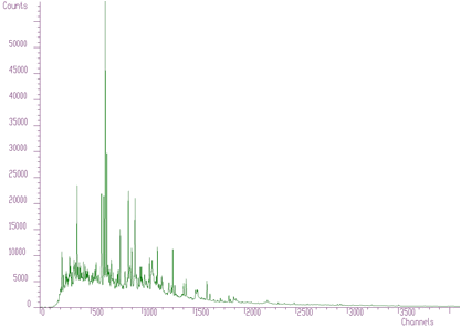
Spectrum with many peaks
In Figures. 6.2, 6.3, 6.4 we present this spectrum transformed using Haar, Walsh and Cosine transforms, respectively.
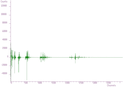
Spectrum transformed using Haar transform
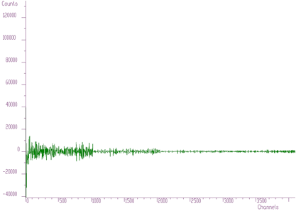
Spectrum transformed using Walsh transform
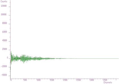
Spectrum transformed using Cosine transform
Haar transforms (Figure 6.2) creates clusters of data. These coefficients can be analyzed and then filtered, enhanced etc. On the other hand Walsh transform (Figure 6.3) concentrates the dominant components near to zero of the coordinate system. It is more suitable to process data of rectangular shape (e.g. in the field of digital signal processing). Finally Cosine transform concentrates in the best way the transform coefficients to the beginning of the coordinate system. From the point of view of the variance distribution it is sometimes called suboptimal. One can notice that approximately one half of the coefficients are negligible. This fact can be utilized to the compression purposes (in two or more dimensional data), filtering (smoothing) etc.
We have implemented several application functions utilizing the properties of the orthogonal transforms. Let us start with zonal filtration function. It has the form.
char *Filter1Zonal(const float *source,
                   float *dest,
                   int size,
                   int type,
                   int degree,
                   int xmin,
                   int xmax,
                   float filter-coeff);
This function transforms the source spectrum. The calling program should fill in input parameters. Then it sets transformed coefficients in the given region (xmin, xmax) to the given filter_coeff and transforms it back Filtered data are written into dest spectrum.
Function parameters:
source pointer to the vector of source spectrum, its length should be sizedest pointer to the vector of dest data, its length should be sizesize basic length of source and dest spectratype type of transform
degree applied only for mixed transformsxmin low limit of filtered regionxmax high limit of filtered regionfilter_coeff value which is set in filtered regionAn example of the filtration using Cosine transform is given in the Figure 6.5. It illustrates a part of the spectrum from Figure 6.1 and two spectra after filtration preserving 2048 coefficients and 1536 coefficients. One can observe very good fidelity of the overall shape of both spectra with the original data. However some distortion can be observed in details of the second spectrum after filtration preserving only 1536 coefficients. The useful information in the transform domain can be compressed into one half of the original space.
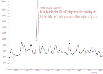
Filtration using Cosine transform
In the transform domain one can also enhance (multiply with the constant > 1) some regions. In this way one can change peak-to-background ratio. This function has the form
char *Enhance1(const float *source,
               float *dest,
               int size,
               int type,
               int degree,
               int xmin,
               int xmax,
               float enhance-coeff);
This function transforms the source spectrum. The calling program should fill in input parameters. Then it multiplies transformed coefficients in the given region (xmin, xmax) by the given enhance_coeff and transforms it back Processed data are written into dest spectrum.
Function parameters:
source pointer to the vector of source spectrum, its length should be sizedest pointer to the vector of dest data, its length should be sizesize basic length of source and dest spectratype type of transform
degree applied only for mixed transformsxmin low limit of filtered regionxmax high limit of filtered regionenhance_coeff value by which the filtered region is multipliedAn example of enhancement of the coefficients from region 380-800 by the constant 2 in the Cosine transform domain is given in the Figure 6.6. The determination of the region is a matter of analysis in the appropriate transform domain. We assumed that low frequency components are placed in the low coefficients. As it can be observed the enhancement changes the peak-to-background ratio.
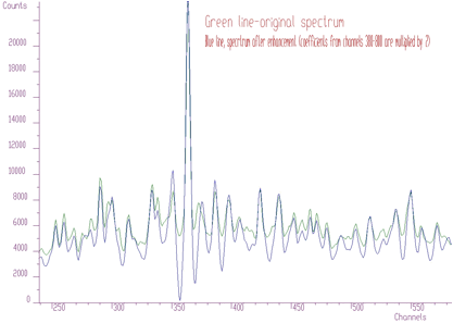
Enhancement of the coefficients from region 380-800 by the constant 2 in the Cosine transform domain
Analogously to1-dimensional data we have implemented the transforms also for 2-dimensional data. Besides of the classic orthogonal transforms
char *Transform2(const float **source,
                 float **dest,
                 int sizex,
                 int sizey,
                 int type,
                 int direction,
                 int degree);
This function transforms the source spectrum. The calling program should fill in input parameters. Transformed data are written into dest spectrum.
Function parameters:
source pointer to the matrix of source spectrum, its size should be sizex*sizey except for inverse FOURIER, FOUR-WALSH, FOUR-HAAR transform. These need sizex*2*sizey length to supply real and imaginary coefficients.dest pointer to the matrix of destination data, its size should be sizex*sizey except for direct FOURIER, FOUR-WALSh, FOUR-HAAR. These need sizex*2*sizey length to store real and imaginary coefficientssizex,sizey basic dimensions of source and dest spectratype type of transform
direction transform direction (forward, inverse)degree applies only for mixed transformsAn example of the 2-dimensional Cosine transform of data from Figure 5.6 is given in Figure 6.7. One can notice that the data are concentrated again around the beginning of the coordinate system. This allows to apply filtration, enhancement and compression techniques in the transform domain.
2-dimensional Cosine transform of data from Figure 5.6
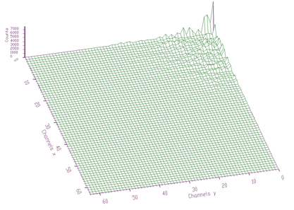
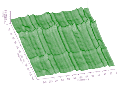
In some cases when the spectrum is smooth the cosine transforms are very efficient. In Figures 6.8, 6.9 we show original spectrum and transformed coefficients using Cosine transform, respectively.
Original spectrum
Transformed coefficients using Cosine transform
Analogously to 1-dimensional case we have implemented also the functions for zonal filtration, Gauss filtration and enhancement. The zonal filtration function using classic transforms has the form
char *Filter2Zonal(const float **source,
                   float **dest,
                   int sizex,
                   int sizey,
                   int type,
                   int degree,
                   int xmin,
                   int xmax,
                   int ymin,
                   int ymax,
                   float filter-coeff);
This function transforms the source spectrum. The calling program should fill in input parameters. Then it sets transformed coefficients in the given region to the given filter_coeff and transforms it back Filtered data are written into dest spectrum.
Function parameters:
source pointer to the matrix of source spectrum, its size should be sizex*sizeydest pointer to the matrix of destination data, its size should be sizex*sizeysizex,sizey basic dimensions of source and dest spectratype type of transform
degree applies only for mixed transformsxmin low limit x of filtered regionxmax high limit x of filtered regionymin low limit y of filtered regionymax high limit y of filtered regionfilter_coeff value which is set in filtered regionThe enhancement function using transforms has the form
char *Enhance2(const float **source,
               float **dest,
               int sizex,
               int sizey,
               int type,
               int degree,
               int xmin,
               int xmax,
               int ymin,
               int ymax,
               float enhance-coeff);
This function transforms the source spectrum. The calling program should fill in input parameters. Then it multiplies transformed coefficients in the given region by the given enhance_coeff and transforms it back
Function parameters:
source pointer to the matrix of source spectrum, its size should be sizex*sizeydest pointer to the matrix of destination data, its size should be sizex*sizeysizex,sizey basic dimensions of source and dest spectratype type of transform
degree applies only for mixed transformsxmin low limit x of filtered regionxmax high limit x of filtered regionymin low limit y of filtered regionymax high limit y of filtered regionenhance-coeff value which is set in filtered regionThe 1-dimensional visualization function displays spectrum (or part of it) on the Canvas of a form. Before calling the function one has to fill in one_dim_pic structure containing all parameters of the display. The function has the form
char *display1(struct one-dim-pic* p);This function displays the source spectrum on Canvas. All parameters are grouped in one_dim_pic structure. Before calling display1 function the structure should be filled in and the address of one_dim_pic passed as parameter to display1 function. The meaning of appropriate parameters is apparent from description of one_dim_pic structure. The constants , which can be used for appropriate parameters are defined in procfunc.h header file.
struct one_dim_pic {

   float *source; // spectrum to be displayed

   TCanvas *Canvas; // Canvas where the spectrum will be displayed

   int size; // size of source spectrum
   int xmin; // x-starting channel of spectrum
   int xmax; // x-end channel of spectrum
   int ymin; // base counts
   int ymax; // count full scale

   int bx1; // position of picture on Canvas, min x
   int bx2; // position of picture on Canvas, max x
   int by1; // position of picture on Canvas, min y
   int by2; // position of picture on Canvas, max y

   int display_mode;    // spectrum display mode (points, polyline, bars, rainbow, steps, bezier)
   int y_scale;         // y scale (linear, log, sqrt)
   int levels;          // # of color levels for rainbow display mode, it does not apply
                        // for other display modes
   float rainbow1_step; // determines the first color component step for neighbouring
                        // color levels, applies only for rainbow display mode
   float rainbow2_step; // determines the second component color step for
                        // neighbouring color levels, applies only for rainbow display mode
   float rainbow3_step; // determines the third component color step for
                        // neighbouring color levels, applies only for rainbow display mode

   int color_alg; // applies only for rainbow display mode (rgb smooth algorithm, rgb
                  // modulo color component, cmy smooth algorithm, cmy modulo color
                  // component, cie smooth algorithm, cie modulo color component, yiq
                  // smooth algorithm, yiq modulo color component, hsv smooth
                  // algorithm, hsv modulo color component [15]

   int bar_thickness;          // applies only for bar display mode
   int bar_empty_flag;         // (empty bars, full bars) applies only for bar display mode
   int border_color;           // color of background of the picture
   int full_border;            // decides whether background is painted
   int raster_en_dis;          // decides whether the axes and rasters are shown
   int raster_long;            // decides whether the rasters are drawn as long lines
   int raster_color;           // color of the rasters
   char *raster_description_x; // x axis description
   char *raster_description_y; // y axis description

   int pen_color; // color of spectrum
   int pen_dash;  // style of pen
   int pen_width; // width of line

   int chanmark_style;  // style of channel marks
   int chanmark_width;  // width of channel marks
   int chanmark_height; // height of channel marks
   int chanmark_en_dis; // decides whether the channel marks are shown
   int chanmark_color;  // color of channel marks

   // auxiliary variables, transform coefficients, for internal use only
   double mx;
   double my;
   double px;
   double py;

   // auxiliary internal variables, working place
   double gbezx,gbezy;
   TPoint bz[4];
};
The examples using different display parameters are shown in the next few Figures
Display mode -polyline, width of pen=3
Display mode- bars, shown channel marks
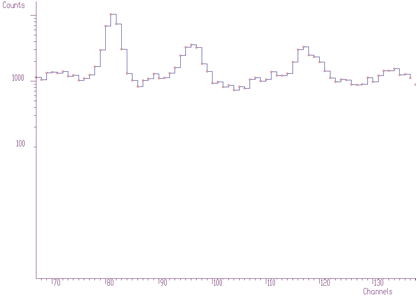
Display mode- steps, log scale, shown channel marks
Display mode -Bezier curve interpolation, shown channel marks
Display mode- rainbow bars, color algorithm (model) RGB, number of color levels=1024, pen width=3
Display mode-empty bars, color algorithm YIQ, number of color levels 2048
The 2-dimensional visualization function displays spectrum (or part of it) on the Canvas of a form. Before calling the function one has to fill in two_dim_pic structure containing all parameters of the display. The function has the form
char *display2(struct two-dim-pic* p);This function displays the source two dimensional spectrum on Canvas. All parameters are grouped in two_dim_pic structure. Before calling display2 function the structure should be filled in and the address of two_dim_pic passed as parameter to display2 function. The meaning of appropriate parameters is apparent from description of one_dim_pic structure. The constants , which can be used for appropriate parameters are defined in procfunc.h header file.
struct two_dim_pic {

   float **source;      // source spectrum to be displayed

   TCanvas *Canvas;     // Canvas where the spectrum will be displayed

   int sizex;           // x-size of source spectrum
   int sizey;           // y-size of source spectrum
   int xmin;            // x-starting channel of spectrum
   int xmax;            // x-end channel of spectrum
   int ymin;            // y-starting channel of spectrum
   int ymax;            // y-end channel of spectrum
   int zmin;            // base counts
   int zmax;            // counts full scale
   int bx1;             // position of picture on Canvas, min x
   int bx2;             // position of picture on Canvas, max x
   int by1;             // position of picture on Canvas, min y
   int by2;             // position of picture on Canvas, max y
   int mode_group;      // display mode algorithm group (simple modes-
                        // PICTURE2_MODE_GROUP_SIMPLE, modes with shading
                        // according to light-PICTURE2_MODE_GROUP_LIGHT, modes with
                        // shading according to channels counts-
                        // PICTURE2_MODE_GROUP_HEIGHT, modes of combination of
                        // shading according to light and to channels counts-
                        // PICTURE2_MODE_GROUP_LIGHT_HEIGHT)
   int display_mode;    // spectrum display mode (points, grid, contours, bars, x_lines,
                        // y_lines, bars_x, bars_y, needles, surface, triangles)
   int z_scale;         // z scale (linear, log, sqrt)
   int nodesx;          // number of nodes in x dimension of grid
   int nodesy;          // number of nodes in y dimension of grid
   int count_reg;       // width between contours, applies only for contours display mode
   int alfa;            // angles of display,alfa+beta must be less or equal to 90, alpha- angle
                        // between base line of Canvas and left lower edge of picture picture
                        // base plane
   int beta;            // angle between base line of Canvas and right lower edge of picture base plane
   int view_angle;      // rotation angle of the view, it can be 0, 90, 180, 270 degrees
   int levels;          // # of color levels for rainbowed display modes, it does not apply for
                        // simple display modes algorithm group
   float rainbow1_step; // determines the first component step for neighbouring color
                        // levels, applies only for rainbowed display modes, it does not apply
                        // for simple display modes algorithm group
   float rainbow2_step; // determines the second component step for neighbouring
                        // color levels, applies only for rainbowed display modes, it does not
                        // apply for simple display modes algorithm group
   float rainbow3_step; // determines the third component step for neighbouring
                        // color levels, applies only for rainbowed display modes, it does not
                        // apply for simple display modes algorithm group
   int color_alg;       // applies only for rainbowed display modes (rgb smooth algorithm,
                        // rgb modulo color component, cmy smooth algorithm, cmy modulo
                        // color component, cie smooth algorithm, cie modulo color component,
                        // yiq smooth algorithm, yiq modulo color component, hsv smooth
                        // algorithm, hsv modulo color component, it does not apply for simple
                        // display modes algorithm group [15]
   float l_h_weight;    // weight between shading according to fictive light source and
                        // according to channels counts, applies only for
                        // PICTURE2_MODE_GROUP_LIGHT_HEIGHT modes group
   int xlight;          // x position of fictive light source, applies only for rainbowed display
                        // modes with shading according to light
   int ylight;          // y position of fictive light source, applies only for rainbowed display
                        // modes with shading according to light
   int zlight;          // z position of fictive light source, applies only for rainbowed display
                        // modes with shading according to light
   int shadow;          // determines whether shadow will be drawn (no shadow, shadow),
                        // for rainbowed display modes with shading according to light
   int shading;         // determines whether the picture will shaded, smoothed (no shading,
                        // shading), for rainbowed display modes only
   int bezier;          // determines Bezier interpolation (applies only for simple display
                        // modes group for grid, x_lines, y_lines display modes)
   int border_color;           // color of background of the picture
   int full_border;            // decides whether background is painted
   int raster_en_dis;          // decides whether the rasters are shown
   int raster_long;            // decides whether the rasters are drawn as long lines
   int raster_color;           // color of the rasters
   char *raster_description_x; // x axis description
   char *raster_description_y; // y axis description
   char *raster_description_z; // z axis description
   int pen_color;              // color of spectrum
   int pen_dash;               // style of pen
   int pen_width;              // width of line
   int chanmark_en_dis;        // decides whether the channel marks are shown
   int chanmark_style;         // style of channel marks
   int chanmark_width;         // width of channel marks
   int chanmark_height;        // height of channel marks
   int chanmark_color;         // color of channel marks
   int chanline_en_dis;        // decides whether the channel lines (grid) are shown

   // auxiliary variables, transformation coefficients for internal use only
   double kx;
   double ky;
   double mxx;
   double mxy;
   double myx;
   double myy;
   double txx;
   double txy;
   double tyx;
   double tyy;
   double tyz;
   double vx;
   double vy;
   double nu_sli;

   // auxiliary internal variables, working place
   double z,zeq,gbezx,gbezy,dxspline,dyspline;
   int xt,yt,xs,ys,xe,ye,priamka,z_preset_value;
   unsigned short obal[MAXIMUM_XSCREEN_RESOLUTION];
   unsigned short obal_cont[MAXIMUM_XSCREEN_RESOLUTION];
   TPoint bz[4];
};
The examples using different display parameters are shown in the next few Figures.
Display mode-bars, pen width=2
Display mode-triangles, log scale
Display mode-contours
Display mode surface shading according to height
Display mode-surface shading according to light point
Display mode-surface shading according to height+light position with ratio 50:50, CMY color model
Display mode bars shaded according to height
Display mode- surface shading according to light position with shadows

Display mode- surface shading according to height with 10 levels of contours
Display mode- surface shading according to height, sqrt scale, channel marks and lines shown
Display mode- surface shading according to height-contours, rasters allowing to localize interesting parts are shown.
[1] M. Morháč, J. Kliman, V. Matoušek, M. Veselský, I. Turzo.: Background elimination methods for multidimensional gamma-ray spectra. NIM, A401 (1997) 113-132.
[2] C. G Ryan et al.: SNIP, a statistics-sensitive background treatment for the quantitative analysis of PIXE spectra in geoscience applications. NIM, B34 (1988), 396-402.
[3] D. D. Burgess, R. J. Tervo: Background estimation for gamma-ray spectroscopy. NIM 214 (1983), 431-434.
[4] M. Morháč, J. Kliman, V. Matoušek, M. Veselský, I. Turzo.:Identification of peaks in multidimensional coincidence gamma-ray spectra. NIM, A443 (2000) 108-125.
[5] M.A. Mariscotti: A method for identification of peaks in the presence of background and its application to spectrum analysis. NIM 50 (1967), 309-320.
[6] Z.K. Silagadze, A new algorithm for automatic photopeak searches. NIM A 376 (1996), 451.
[7] P. Bandžuch, M. Morháč, J. Krištiak: Study of the VanCitter and Gold iterative methods of deconvolutionand their application in the deconvolution of experimental spectra of positron annihilation, NIM A 384 (1997) 506-515.
[8] M. Morháč, J. Kliman, V. Matoušek, M. Veselský, I. Turzo.: Efficient one- and two-dimensional Gold deconvolution and its application to gamma-ray spectra decomposition. NIM, A401 (1997) 385-408.
[9] I. A. Slavic: Nonlinear least-squares fitting without matrix inversion applied to complex Gaussian spectra analysis. NIM 134 (1976) 285-289.
[10] B. Mihaila: Analysis of complex gamma spectra, Rom. Jorn. Phys., Vol. 39, No. 2, (1994), 139-148.
[11] T. Awaya: A new method for curve fitting to the data with low statistics not using chi-square method. NIM 165 (1979) 317-323.
[12] T. Hauschild, M. Jentschel: Comparison of maximum likelihood estimation and chi-square statistics applied to counting experiments. NIM A 457 (2001) 384-401.
[13] M. Morháč, J. Kliman, M. Jandel, Ľ. Krupa, V. Matoušek: Study of fitting algorithms applied to simultaneous analysis of large number of peaks in \(\gamma\)-ray spectra. Applied spectroscopy, Accepted for publication.
[14] C.V. Hampton, B. Lian, Wm. C. McHarris: Fast-Fourier-transform spectral enhancement techniques for gamma-ray spectroscopy. NIM A353 (1994) 280-284..
[15] D. Hearn, M. P. Baker: Computer Graphics, Prentice-Hall International, Inc., 1994.