

Graphical capabilities of ROOT range from 2D objects (lines, polygons, arrows) to various plots, histograms, and 3D graphical objects. In this chapter, we are going to focus on principals of graphics and 2D objects. Plots and histograms are discussed in a chapter of their own.
In ROOT, most objects derive from a base class TObject. This class has a virtual method Draw() so all objects are supposed to be able to be “drawn”. The basic whiteboard on which an object is drawn is called a canvas (defined by the class TCanvas). If several canvases are defined, there is only one active at a time. One draws an object in the active canvas by using the statement:
object.Draw()This instructs the object “object” to draw itself. If no canvas is opened, a default one (named “c1”) is instantiated and is drawn.
root[] TLine a(0.1,0.1,0.6,0.6)
root[] a.Draw()
<TCanvas::MakeDefCanvas>: created default TCanvas with name c1
The first statement defines a line and the second one draws it. A default canvas is drawn since there was no opened one.
When an object is drawn, one can interact with it. For example, the line drawn in the previous paragraph may be moved or transformed. One very important characteristic of ROOT is that transforming an object on the screen will also transform it in memory. One actually interacts with the real object, not with a copy of it on the screen. You can try for instance to look at the starting X coordinate of the line:
root[] a.GetX1()
(double)1.000000000e-1
X1 is the x value of the starting coordinate given in the definition above. Now move it interactively by clicking with the left mouse button in the line’s middle and try to do again:
root[] a.GetX1()
(Double_t)1.31175468483816005e-01
You do not obtain the same result as before, the coordinates of ‘a’ have changed. As said, interacting with an object on the screen changes the object in memory.
Changing the graphic objects attributes can be done with the GUI or programmatically. First, let’s see how it is done in the GUI.
As was just seen moving or resizing an object is done with the left mouse button. The cursor changes its shape to indicate what may be done:
Point the object or one part of it:
Rotate: 
Resize (exists also for the other directions): 

Enlarge (used for text): 
Move: 
Here are some examples of:
Moving:  Resizing:
Rotating: 

How would one move an object in a script? Since there is a tight correspondence between what is seen on the screen and the object in memory, changing the object changes it on the screen. For example, try to do:
root[] a.SetX1(0.9)This should change one of the coordinates of our line, but nothing happens on the screen. Why is that? In short, the canvas is not updated with each change for performance reasons. See “Updating the Pad”.
Objects in a canvas, as well as in a pad, are stacked on top of each other in the order they were drawn. Some objects may become “active” objects, which mean they are reordered to be on top of the others. To interactively make an object “active”, you can use the middle mouse button. In case of canvases or pads, the border becomes highlighted when it is active.
Frequently we want to draw in different canvases or pads. By default, the objects are drawn in the active canvas. To activate a canvas you can use the TPad::cd() method.
root[] c1->cd()The context menus are a way to interactively call certain methods of an object. When designing a class, the programmer can add methods to the context menu of the object by making minor changes to the header file.
On a ROOT canvas, you can right-click on any object and see the context menu for it. The script hsimple.C draws a histogram. The image below shows the context menus for some of the objects on the canvas. Next picture shows that drawing a simple histogram involves as many as seven objects. When selecting a method from the context menu and that method has options, the user will be asked for numerical values or strings to fill in the option. For example, TAxis::SetTitle will prompt you for a string to use for the axis title.
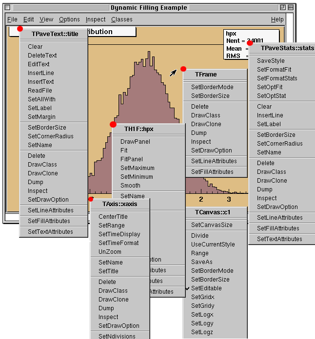
Context menus of different objects in a canvas
The curious reader will have noticed that each entry in the context menu corresponds to a method of the class. Look for example to the menu named TAxis::xaxis. xaxis is the name of the object and TAxis the name of its class. If we look at the list of TAxis methods, for example in http://root.cern.ch/root/htmldoc/TAxis.html, we see the methods SetTimeDisplay() andUnZoom(), which appear also in the context menu.
There are several divisions in the context menu, separated by lines. The top division is a list of the class methods; the second division is a list of the parent class methods. The subsequent divisions are the methods other parent classes in case of multiple inheritance. For example, see the TPaveText::title context menu. A TPaveText inherits from TAttLine, which has the method SetLineAttributes().
For a method to appear in the context menu of the object it has to be marked by // *MENU* in the header file. Below is the line from TAttLine.h that adds the SetLineAttribute method to the context menu.
virtual void SetLineAttributes(); // *MENU*Nothing else is needed, since CINT knows the classes and their methods. It takes advantage of that to create the context menu on the fly when the object is clicking on. If you click on an axis, ROOT will ask the interpreter what are the methods of the TAxis and which ones are set for being displayed in a context menu.
Now, how does the interpreter know this? Remember, when you build a class that you want to use in the ROOT environment, you use rootcint that builds the so-called stub functions and the dictionary. These functions and the dictionary contain the knowledge of the used classes. To do this, rootcint parses all the header files. ROOT has defined some special syntax to inform CINT of certain things, this is done in the comments so that the code still compiles with a C++ compiler.
For example, you have a class with a Draw() method, which will display itself. You would like a context menu to appear when on clicks on the image of an object of this class. The recipe is the following:
The class has to contain the ClassDef/ClassImp macros
For each method you want to appear in the context menu, put a comment after the declaration containing *MENU* or *TOGGLE* depending on the behavior you expect. One usually uses Set methods (setters). The *TOGGLE* comment is used to toggle a boolean data field. In that case, it is safe to call the data field fMyBool where MyBool is the name of the setter SetMyBool. Replace MyBool with your own boolean variable.
You can specify arguments and the data members in which to store the arguments.
For example:
class MyClass : public TObject {
private:
   int      fV1;   // first variable
   double   fV2;   // second variable
public:
   int    GetV1() {return fV1;}
   double GetV2() {return fV2;}
   void   SetV1(int x1) { fV1 = x1;}     // *MENU*
   void   SetV2(double d2) { fV2 = d2;}  // *MENU*
   void   SetBoth(int x1, double d2) {fV1 = x1; fV2 = d2;}

   ClassDef (MyClass,1)
}
To specify arguments:
void SetXXX(Int_t x1, Float_t y2); //*MENU* *ARGS={x1=>fV1}This statement is in the comment field, after the *MENU*. If there is more than one argument, these arguments are separated by commas, where fX1 and fY2 are data fields in the same class.
void SetXXX(Int_t x1, Float_t y2); //*MENU* *ARGS={x1=>fX1,y2=>fY2}If the arguments statement is present, the option dialog displayed when selecting SetXXX field will show the values of variables. We indicate to the system which argument corresponds to which data member of the class.
This paragraph is for class designers. When a class is designed, it is often desirable to include drawing methods for it. We will have a more extensive discussion about this, but drawing an object in a canvas or a pad consists in “attaching” the object to that pad. When one uses object.Draw(), the object is NOT painted at this moment. It is only attached to the active pad or canvas.
Another method should be provided for the object to be painted, the Paint() method. This is all explained in the next paragraph. As well as Draw() and Paint(), other methods may be provided by the designer of the class. When the mouse is moved or a button pressed/released, the TCanvas function named HandleInput() scans the list of objects in all it’s pads and for each object calls some standard methods to make the object react to the event (mouse movement, click or whatever).
The second one is DistanceToPrimitive(px,py). This function computes a “distance” to an object from the mouse position at the pixel position (px, py, see definition at the end of this paragraph) and returns this distance in pixel units. The selected object will be the one with the shortest computed distance. To see how this works, select the “Event Status” item in the canvas “Options” menu. ROOT will display one status line showing the picked object. If the picked object is, for example, a histogram, the status line indicates the name of the histogram, the position x,y in histogram coordinates, the channel number and the channel content.
It is nice for the canvas to know what the closest object from the mouse is, but it’s even nicer to be able to make this object react. The third standard method to be provided is ExecuteEvent(). This method actually does the event reaction. Its prototype is where px and py are the coordinates at which the event occurred, except if the event is a key press, in which case px contains the key code.
void ExecuteEvent(Int_t event, Int_t px, Int_t py);Where event is the event that occurs and is one of the following (defined in Buttons.h):
kNoEvent,          kButton1Down,      kButton2Down,
kButton3Down,      kKeyDown,          kButton1Up,
kButton2Up,        kButton3Up,        kButton1Motion,
kButton2Motion,    kButton3Motion,    kKeyPress,
kButton1Locate,    kButton2Locate,    kButton3Locate,
kKeyUp,            kButton1Double,    kButton2Double,
kButton3Double,    kMouseMotion,      kMouseEnter,
kMouseLeave
We hope the names are self-explanatory.
Designing an ExecuteEvent method is not very easy, except if one wants very basic treatment. We will not go into that and let the reader refer to the sources of classes like TLine or TBox. Go and look at their ExecuteEvent method! We can nevertheless give some reference to the various actions that may be performed. For example, one often wants to change the shape of the cursor when passing on top of an object. This is done with the SetCursor method:
gPad->SetCursor(cursor)The argument cursor is the type of cursor. It may be:
kBottomLeft,  kBottomRight,  kTopLeft,
kTopRight,    kBottomSide,   kLeftSide,
kTopSide,     kRightSide,    kMove,
kCross,       kArrowHor,     kArrowVer,
kHand,        kRotate,       kPointer,
kArrowRight,  kCaret,        kWatch
They are defined in TVirtualX.h and again we hope the names are self-explanatory. If not, try them by designing a small class. It may derive from something already known like TLine.
Note that the ExecuteEvent() functions may in turn; invoke such functions for other objects, in case an object is drawn using other objects. You can also exploit at best the virtues of inheritance. See for example how the class TArrow (derived from TLine) use or redefine the picking functions in its base class.
The last comment is that mouse position is always given in pixel units in all these standard functions. px=0 and py=0 corresponds to the top-left corner of the canvas. Here, we have followed the standard convention in windowing systems. Note that user coordinates in a canvas (pad) have the origin at the bottom-left corner of the canvas (pad). This is all explained in the paragraph “The Coordinate Systems of a Pad”.
We have talked a lot about canvases, which may be seen as windows. More generally, a graphical entity that contains graphical objects is called a Pad. A Canvas is a special kind of Pad. From now on, when we say something about pads, this also applies to canvases. A pad (class TPad) is a graphical container in the sense it contains other graphical objects like histograms and arrows. It may contain other pads (sub-pads) as well. A Pad is a linked list of primitives of any type (graphs, histograms, shapes, tracks, etc.). It is a kind of display list.

The pad display list
Drawing an object is nothing more than adding its pointer to this list. Look for example at the code of TH1::Draw(). It is merely ten lines of code. The last statement is AppendPad(). This statement calls method of TObject that just adds the pointer of the object, here a histogram, to the list of objects attached to the current pad. Since this is a TObject’s method, every object may be “drawn”, which means attached to a pad.
When is the painting done then ? The answer is: when needed. Every object that derives from TObject has a Paint() method. It may be empty, but for graphical objects, this routine contains all the instructions to paint effectively it in the active pad. Since a Pad has the list of objects it owns, it will call successively the Paint() method of each object, thus re-painting the whole pad on the screen. If the object is a sub-pad, its Paint() method will call the Paint() method of the objects attached, recursively calling Paint() for all the objects.
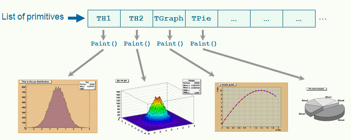
Pad painting
In some cases a pad need to be painted during a macro execution. To force the pad painting gPad->Update() (see next section) should be performed.
The list of primitives stored in the pad is also used to pick objects and to interact with them.
When an object is drawn, it is always in the so-called active pad. For every day use, it is comfortable to be able to access the active pad, whatever it is. For that purpose, there is a global pointer, called gPad. It is always pointing to the active pad. If you want to change the fill color of the active pad to blue but you do not know its name, do this.
root[] gPad->SetFillColor(38)To get the list of colors, go to the paragraph “Color and color palettes” or if you have an opened canvas, click on the View menu, selecting the Colors item.
Now that we have a pointer to the active pad, gPad and that we know this pad contains some objects, it is sometimes interesting to access one of those objects. The method GetPrimitive() of TPad, i.e. TPad::GetPrimitive(const char* name) does exactly this. Since most of the objects that a pad contains derive from TObject, they have a name. The following statement will return a pointer to the object myobjectname and put that pointer into the variable obj. As you can see, the type of returned pointer is TObject*.
root[] obj = gPad->GetPrimitive("myobjectname")
(class TObject*)0x1063cba8
Even if your object is something more complicated, like a histogram TH1F, this is normal. A function cannot return more than one type. So the one chosen was the lowest common denominator to all possible classes, the class from which everything derives, TObject. How do we get the right pointer then? Simply do a cast of the function output that will transform the output (pointer) into the right type. For example if the object is a TPaveLabel:
root[] obj = (TPaveLabel*)(gPad->GetPrimitive("myobjectname"))
(class TPaveLabel*)0x1063cba8
This works for all objects deriving from TObject. However, a question remains. An object has a name if it derives from TNamed, not from TObject. For example, an arrow (TArrow) doesn’t have a name. In that case, the “name” is the name of the class. To know the name of an object, just click with the right button on it. The name appears at the top of the context menu. In case of multiple unnamed objects, a call to GetPrimitive("className") returns the instance of the class that was first created. To retrieve a later instance you can use GetListOfPrimitives(), which returns a list of all the objects on the pad. From the list you can select the object you need.
Hiding an object in a pad can be made by removing it from the list of objects owned by that pad. This list is accessible by the GetListOfPrimitives() method of TPad. This method returns a pointer to a TList. Suppose we get the pointer to the object, we want to hide, call it obj (see paragraph above). We get the pointer to the list:
root[] li = gPad->GetListOfPrimitives()Then remove the object from this list:
root[] li->Remove(obj)The object will disappear from the pad as soon as the pad is updated (try to resize it for example). If one wants to make the object reappear:
root[] obj->Draw()Caution, this will not work with composed objects, for example many histograms drawn on the same plot (with the option “same”). There are other ways! Try to use the method described here for simple objects.
There are coordinate systems in a TPad: user coordinates, normalized coordinates (NDC), and pixel coordinates.
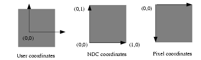
Pad coordinate systems
The most common is the user coordinate system. Most methods of TPad use the user coordinates, and all graphic primitives have their parameters defined in terms of user coordinates. By default, when an empty pad is drawn, the user coordinates are set to a range from 0 to 1 starting at the lower left corner. At this point they are equivalent of the NDC coordinates (see below). If you draw a high level graphical object, such as a histogram or a function, the user coordinates are set to the coordinates of the histogram. Therefore, when you set a point it will be in the histogram coordinates.
For a newly created blank pad, one may use TPad::Range to set the user coordinate system. This function is defined as:
void Range(float x1,float y1,float x2,float y2)The arguments x1, x2 defines the new range in the x direction, and the y1, y2 define the new range in the y-direction.
root[] TCanvas MyCanvas ("MyCanvas")
root[] gPad->Range(-100,-100,100,100)
This will set the active pad to have both coordinates to go from -100 to 100, with the center of the pad at (0,0). You can visually check the coordinates by viewing the status bar in the canvas. To display the status bar select Event Status entry in the View canvas menu.
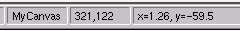
The status bar
Normalized coordinates are independent of the window size and of the user system. The coordinates range from 0 to 1 and (0, 0) corresponds to the bottom-left corner of the pad. Several internal ROOT functions use the NDC system (3D primitives, PostScript, log scale mapping to linear scale). You may want to use this system if the user coordinates are not known ahead of time.
The least common is the pixel coordinate system, used by functions such as DistanceToPrimitive() and ExecuteEvent(). Its primary use is for cursor position, which is always given in pixel coordinates. If (px,py) is the cursor position, px=0 and py=0 corresponds to the top-left corner of the pad, which is the standard convention in windowing systems.
Most of the time, you will be using the user coordinate system. But sometimes, you will want to use NDC. For example, if you want to draw text always at the same place over a histogram, no matter what the histogram coordinates are. There are two ways to do this. You can set the NDC for one object or may convert NDC to user coordinates. Most graphical objects offer an option to be drawn in NDC. For instance, a line (TLine) may be drawn in NDC by using DrawLineNDC(). A latex formula or a text may use TText::SetNDC() to be drawn in NDC coordinates.
There are a few utility functions in TPad to convert from one system of coordinates to another. In the following table, a point is defined by (px,py) in pixel coordinates, (ux,uy) in user coordinates, (ndcx,ndcy) in normalized coordinates, (apx, apy) are in absolute pixel coordinates.
Conversion |
TPad’s Methods |
Returns |
NDC to Pixel |
|
Int_t Int_t |
Pixel to User |
|
Double_t Double_t Double_t ux,uy |
User to Pixel |
|
Int_t Int_t Int_t px,py |
User to absolute pixel |
|
Int_t Int_t Int_t apx,apy |
Absolute pixel to user |
|
Double_t Double_t Double_t ux,uy |
Note: all the pixel conversion functions along the Y axis consider that py=0 is at the top of the pad except PixeltoY() which assume that the position py=0 is at the bottom of the pad. To make PixeltoY() converting the same way as the other conversion functions, it should be used the following way (p is a pointer to a TPad):
p->PixeltoY(py - p->GetWh());Dividing a pad into sub pads in order for instance to draw a few histograms, may be done in two ways. The first is to build pad objects and to draw them into a parent pad, which may be a canvas. The second is to automatically divide a pad into horizontal and vertical sub pads.
The simplest way to divide a pad is to build sub-pads in it. However, this forces the user to explicitly indicate the size and position of those sub-pads. Suppose we want to build a sub-pad in the active pad (pointed by gPad). First, we build it, using a TPad constructor:
root[] spad1 = new TPad("spad1","The first subpad",.1,.1,.5,.5)One gives the coordinates of the lower left point (0.1, 0.1) and of the upper right one (0.5, 0.5). These coordinates are in NDC. This means that they are independent of the user coordinates system, in particular if you have already drawn for example a histogram in the mother pad. The only thing left is to draw the pad:
root[] spad1->Draw()If you want more sub-pads, you have to repeat this procedure as many times as necessary.
The manual way of dividing a pad into sub-pads is sometimes very tedious. There is a way to automatically generate horizontal and vertical sub-pads inside a given pad.
root[] pad1->Divide(3,2)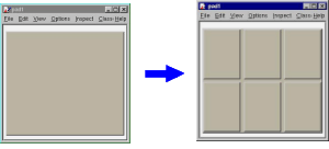
Dividing a pad into 6 sub-pads
Dividing a pad into 6 sub-pads
If pad1 is a pad then, it will divide the pad into 3 columns of 2 sub-pads. The generated sub-pads get names pad1_i where the index i=1 to nxm (in our case pad1_1, pad1_2…pad1_6). The names pad1_1etc… correspond to new variables in CINT, so you may use them as soon as the executed method was pad->Divide(). However, in a compiled program, one has to access these objects. Remember that a pad contains other objects and that these objects may themselves be pads. So we can use the GetPrimitive() method:
TPad* pad1_1 = (TPad*)(pad1->GetPrimitive("pad1_1"))One question remains. In case one does an automatic divide, how one can set the default margins between pads? This is done by adding two parameters to Divide(), which are the margins in x and y:
root[] pad1->Divide(3,2,0.1,0.1)The margins are here set to 10% of the parent pad width.
For performance reasons, a pad is not updated with every change. For example, changing the coordinates of the pad does not automatically redraw it. Instead, the pad has a “bit-modified” that triggers a redraw. This bit is automatically set by:
Touching the pad with the mouse - for example resizing it with the mouse.
Finishing the execution of a script.
Adding a new primitive or modifying some primitives for example the name and title of an object.
You can also set the “bit-modified” explicitly with the Modified method:
// the pad has changed
root[] pad1->Modified()
// recursively update all modified pads:
root[] c1->Update()
A subsequent call to TCanvas::Update() scans the list of sub-pads and repaints the pads declared modified.
In compiled code or in a long macro, you may want to access an object created during the paint process. To do so, you can force the painting with a TCanvas::Update(). For example, a TGraph creates a histogram (TH1) to paint itself. In this case the internal histogram obtained with TGraph::GetHistogram() is created only after the pad is painted. The pad is painted automatically after the script is finished executing or if you force the painting with TPad::Modified() followed by a TCanvas::Update(). Note that it is not necessary to call TPad::Modified() after a call to Draw(). The “bit-modified” is set automatically by Draw(). A note about the “bit-modified” in sub pads: when you want to update a sub pad in your canvas, you need to call pad->Modified() rather than canvas->Modified(), and follow it with a canvas->Update(). If you use canvas->Modified(), followed by a call to canvas->Update(), the sub pad has not been declared modified and it will not be updated. Also note that a call to pad->Update() where pad is a sub pad of canvas, calls canvas->Update() and recursively updates all the pads on the canvas.
As we will see in the paragraph “Fill Attributes”, a fill style (type of hatching) may be set for a pad.
root[] pad1->SetFillStyle(istyle)This is done with the SetFillStyle method where istyle is a style number, defined in “Fill Attributes”. A special set of styles allows handling of various levels of transparency. These are styles number 4000 to 4100, 4000 being fully transparent and 4100 fully opaque. So, suppose you have an existing canvas with several pads. You create a new pad (transparent) covering for example the entire canvas. Then you draw your primitives in this pad. The same can be achieved with the graphics editor. For example:
root[] .x tutorials/hist/h1draw.C
root[] TPad *newpad=new TPad("newpad","Transparent pad",0,0,1,1);
root[] newpad->SetFillStyle(4000);
root[] newpad->Draw();
root[] newpad->cd();
root[] // create some primitives, etcSetting the scale to logarithmic or linear is an attribute of the pad, not the axis or the histogram. The scale is an attribute of the pad because you may want to draw the same histogram in linear scale in one pad and in log scale in another pad. Frequently, we see several histograms on top of each other in the same pad. It would be very inconvenient to set the scale attribute for each histogram in a pad.
Furthermore, if the logic was set in the histogram class (or each object) the scale setting in each Paint method of all objects should be tested.
If you have a pad with a histogram, a right-click on the pad, outside of the histograms frame will convince you. The SetLogx(), SetLogy() and SetLogz() methods are there. As you see, TPad defines log scale for the two directions x and y plus z if you want to draw a 3D representation of some function or histogram.
The way to set log scale in the x direction for the active pad is:
root[] gPad->SetLogx(1)To reset log in the z direction:
root[] gPad->SetLogz(0)If you have a divided pad, you need to set the scale on each of the sub-pads. Setting it on the containing pad does not automatically propagate to the sub-pads. Here is an example of how to set the log scale for the x-axis on a canvas with four sub-pads:
root[] TCanvas MyCanvas("MyCanvas","My Canvas")
root[] MyCanvas->Divide(2,2)
root[] MyCanvas->cd(1)
root[] gPad->SetLogx()
root[] MyCanvas->cd(2)
root[] gPad->SetLogx()
root[] MyCanvas->cd(3)
root[] gPad->SetLogx()When the TPad::WaitPrimitive() method is called with no arguments, it will wait until a double click or any key pressed is executed in the canvas. A call to gSystem->Sleep(10) has been added in the loop to avoid consuming at all the CPU. This new option is convenient when executing a macro. By adding statements like:
canvas->WaitPrimitive();You can monitor the progress of a running macro, stop it at convenient places with the possibility to interact with the canvas and resume the execution with a double click or a key press.
You can make the TPad non-editable. Then no new objects can be added, and the existing objects and the pad can not be changed with the mouse or programmatically. By default the TPad is editable.
TPad::SetEditable(kFALSE)In this paragraph, we describe the various simple 2D graphical objects defined in ROOT. Usually, one defines these objects with their constructor and draws them with their Draw() method. Therefore, the examples will be very brief. Most graphical objects have line and fill attributes (color, width) that will be described in “Graphical objects attributes”. If the user wants more information, the class names are given and he may refer to the online developer documentation. This is especially true for functions and methods that set and get internal values of the objects described here. By default 2D graphical objects are created in User Coordinates with (0, 0) in the lower left corner.
The simplest graphical object is a line. It is implemented in the TLine class. The line constructor is:
TLine(Double_t x1,Double_t y1,Double_t x2,Double_t y2)The arguments x1, y1, x2, y2 are the coordinates of the first and second point. It can be used:
root[] l = new TLine(0.2,0.2,0.8,0.3)
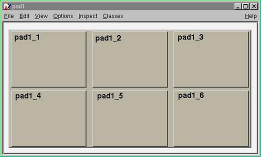
root[] l->Draw()The arrow constructor is:
TArrow(Double_t x1, Double_t y1,
       Double_t x2, Double_t y2,
       Float_t arrowsize, Option_t *option)
It defines an arrow between points x1,y1 and x2,y2. The arrow size is in percentage of the pad height. The option parameter has the following meanings:
 “>”
“>”
 “<|”
“<|”
 “<”
“<”
 “|>”
“|>”
 “<>”
“<>”
 “<|>”
“<|>”
Once an arrow is drawn on the screen, one can:
click on one of the edges and move this edge.
click on any other arrow part to move the entire arrow.
Different arrow formats
If FillColor is 0, an open triangle is drawn; else a full triangle is filled with the set fill color. If ar is an arrow object, fill color is set with:
ar.SetFillColor(icolor);Where icolor is the color defined in “Color and Color Palettes”.
The default-opening angle between the two sides of the arrow is 60 degrees. It can be changed with the method ar->SetAngle(angle), where angle is expressed in degrees.
A poly-line is a set of joint segments. It is defined by a set of N points in a 2D space. Its constructor is:
TPolyLine(Int_t n,Double_t* x,Double_t* y,Option_t* option)Where n is the number of points, and x and y are arrays of n elements with the coordinates of the points. TPolyLine can be used by it self, but is also a base class for other objects, such as curly arcs.
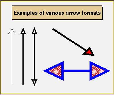
An ellipse can be truncated and rotated. It is defined by its center (x1,y1) and two radii r1 and r2. A minimum and maximum angle may be specified (phimin,phimax). The ellipse may be rotated with an angle theta. All these angles are in degrees. The attributes of the outline line are set via TAttLine, of the fill area - via TAttFill class. They are described in “Graphical Objects Attributes”.
Different types of ellipses
When an ellipse sector is drawn only, the lines between the center and the end points of the sector are drawn by default. By specifying the drawn option “only”, these lines can be avoided. Alternatively, the method SetNoEdges() can be called. To remove completely the ellipse outline, specify zero (0) as a line style.
The TEllipse constructor is:
TEllipse(Double_t x1, Double_t y1, Double_t r1, Double_t r2,
         Double_t phimin, Double_t phimax, Double_t theta)
An ellipse may be created with:
root[] e = new TEllipse(0.2,0.2,0.8,0.3)
root[] e->Draw()The class TBox defines a rectangle. It is a base class for many different higher-level graphical primitives. Its bottom left coordinates x1, y1 and its top right coordinates x2, y2, defines a box. The constructor is:
TBox(Double_t x1,Double_t y1,Double_t x2,Double_t y2)It may be used as in:
root[] b = new TBox(0.2,0.2,0.8,0.3)
root[] b->SetFillColor(5)
root[] b->Draw()
A rectangle with a border
A TWbox is a rectangle (TBox) with a border size and a border mode. The attributes of the outline line and of the fill area are described in “Graphical Objects Attributes”
A marker is a point with a fancy shape! The possible markers are shown in the next figure.
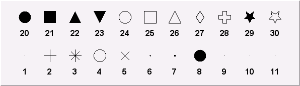
Markers
The marker constructor is:
TMarker(Double_t x,Double_t y,Int_t marker)The parameters x and y are the marker coordinates and marker is the marker type, shown in the previous figure. Suppose the pointer ma is a valid marker. The marker size is set via ma->SetMarkerSize(size), where size is the desired size. Note, that the marker types 1, 6 and 7 (the dots) cannot be scaled. They are always drawn with the same number of pixels. SetMarkerSize does not apply on them. To have a “scalable dot” a circle shape should be used instead, for example, the marker type 20. The default marker type is 1, if SetMarkerStyle is not specified. It is the most common one to draw scatter plots.
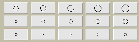
Different marker sizes
Different marker sizes
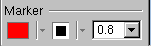
The user interface for changing the marker color, style and size looks like shown in this picture. It takes place in the editor frame anytime the selected object inherits the class TAttMarker.
Non-symmetric symbols should be used carefully in plotting. The next two graphs show how the misleading a careless use of symbols can be. The two plots represent the same data sets but because of a bad symbol choice, the two on the top appear further apart from the next example.
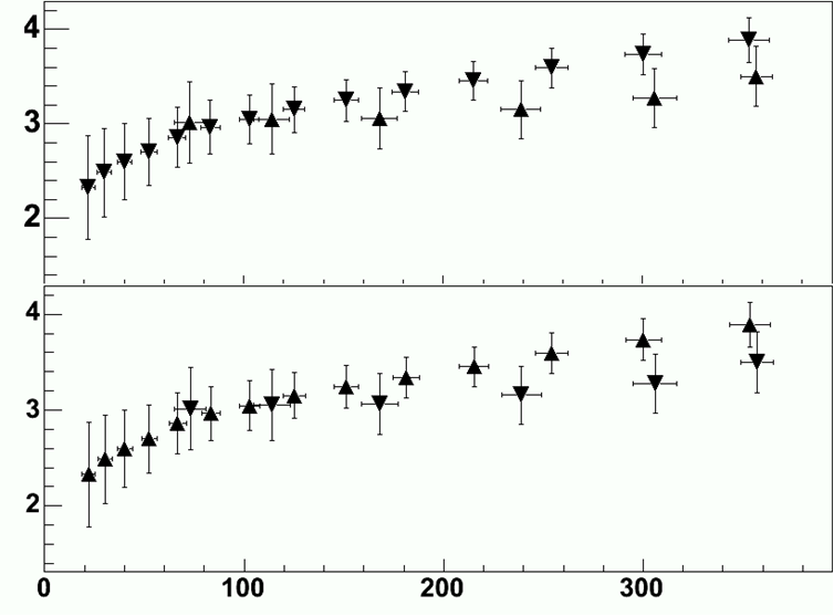
The use of non-symmetric markers
A TPolyMaker is defined by an array on N points in a 2D space. At each point x[i], y[i] a marker is drawn. The list of marker types is shown in the previous paragraph. The marker attributes are managed by the class TAttMarker and are described in “Graphical Objects Attributes”. The TPolyMarker constructor is:
TPolyMarker(Int_t n,Double_t *x,Double_t *y,Option_t *option)Where x and y are arrays of coordinates for the n points that form the poly-marker.
This is a peculiarity of particle physics, but we do need sometimes to draw Feynman diagrams. Our friends working in banking can skip this part. A set of classes implements curly or wavy poly-lines typically used to draw Feynman diagrams. Amplitudes and wavelengths may be specified in the constructors, via commands or interactively from context menus. These classes are TCurlyLine and TCurlyArc. These classes make use of TPolyLine by inheritance; ExecuteEvent methods are highly inspired from the methods used in TPolyLine and TArc.
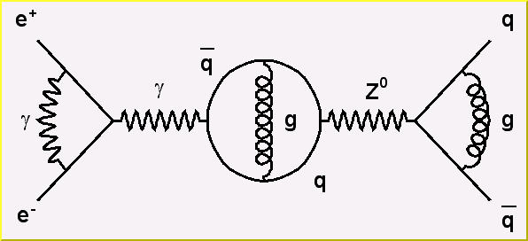
The picture generated by the tutorial macro feynman.C
The TCurlyLine constructor is:
TCurlyLine(Double_t x1, Double_t y1, Double_t x2, Double_t y2,
           Double_t wavelength, Double_t amplitude)
The coordinates (x1, y1) define the starting point, (x2, y2) - the end-point. The wavelength and the amplitude are given in percent of the pad height.
The TCurlyArc constructor is:
TCurlyArc(Double_t x1, Double_t y1, Double_t rad,
          Double_t phimin, Double_t phimax,
          Double_t wavelength, Double_t amplitude)
The curly arc center is (x1, y1) and the radius is rad. The wavelength and the amplitude are given in percent of the line length. The parameters phimin and phimax are the starting and ending angle of the arc (given in degrees). Refer to $ROOTSYS/tutorials/graphics/feynman.C for the script that built the figure above.
Text displayed in a pad may be embedded into boxes, called paves (TPaveLabel), or titles of graphs or many other objects but it can live a life of its own. All text displayed in ROOT graphics is an object of class TText. For a physicist, it will be most of the time a TLatex expression (which derives from TText). TLatex has been conceived to draw mathematical formulas or equations. Its syntax is very similar to the Latex in mathematical mode.
Subscripts and superscripts are made with the _ and ^ commands. These commands can be combined to make complex subscript and superscript expressions. You may choose how to display subscripts and superscripts using the 2 functions SetIndiceSize(Double_t) and SetLimitIndiceSize(Int_t). Examples of what can be obtained using subscripts and superscripts:
The expression |
Gives |
The expression |
Gives |
The expression |
Gives |
|
\(x^{2y}\) |
|
\(x^{y^{2}}\) |
|
\(x_{1}^{y_{1}}\) |
|
\(x_{2y}\) |
|
\(x^{y_{1}}\) |
|
\(x_{1}^{y}\) |
Fractions denoted by the / symbol are made in the obvious way. The #frac command is used for large fractions in displayed formula; it has two arguments: the numerator and the denominator. For example, the equation x = y + z 2 y 2 + 1 is obtained by following expression x=#frac{y+z/2}{y^{2}+1}.
The #sqrt command produces the square ROOT of its argument; it has an optional first argument for other roots.
Example: #sqrt{10} #sqrt[3]{10} 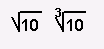
You can produce three kinds of proportional delimiters.
#[]{....} or “à la” Latex
#left[.....#right]big square brackets
#{}{....} or #left{.....#right}big curly brackets
#||{....} or #left|.....#right|big absolute value symbol
#(){....} or #left(.....#right)big parenthesis
You can change the font and the text color at any moment using:
#font[font-number]{...} and #color[color-number]{...}
A TLatex string may be split in two with the following command: #splitline{top}{bottom}. TAxis and TGaxis objects can take advantage of this feature. For example, the date and time could be shown in the time axis over two lines with: #splitline{21 April 2003}{14:23:56}
The command to produce a lowercase Greek letter is obtained by adding # to the name of the letter. For an uppercase Greek letter, just capitalize the first letter of the command name.
#alpha     #beta    #chi      #delta     #varepsilon  #phi
#gamma     #eta     #iota     #varphi    #kappa       #lambda
#mu        #nu      #omicron  #pi        #theta       #rho
#sigma     #tau     #upsilon  #varomega  #omega       #xi
#psi       #zeta    #Alpha    #Beta      #Chi         #Delta
#Epsilon   #Phi     #Gamma    #Eta       #Iota        #Kappa
#vartheta  #Lambda  #Mu       #Nu        #Omicron     #Pi
#Theta     #Rho     #Sigma    #Tau       #Upsilon     #Omega
#varsigma  #Xi      #Psi      #epsilon   #varUpsilon  #Zeta
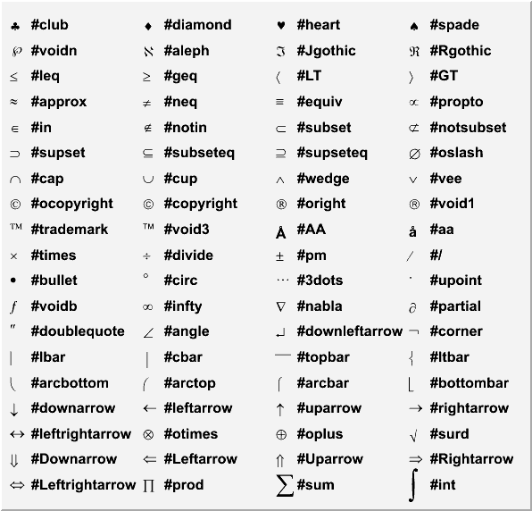
TLatex can make mathematical and other symbols. A few of them, such as + and >, are produced by typing the corresponding keyboard character. Others are obtained with the commands as shown in the table above.
Symbols in a formula are sometimes placed one above another. TLatex provides special commands for that.
#hat{a} =hat
#check =inverted hat
#acute =acute
#grave =accent grave
#dot =derivative
#ddot =double derivative
#tilde =tilde
#slash =special sign. Draw a slash on top of the text between brackets for example
#slash{E}_{T}generates “Missing ET”
a _ is obtained with #bar{a}
a -> is obtained with #vec{a}
The script $ROOTSYS/tutorials/graphics/latex.C:
{
  TCanvas c1("c1","Latex",600,700);
  TLatex l;
  l.SetTextAlign(12);
  l.SetTextSize(0.04);

  l.DrawLatex(0.1,0.8,"1) C(x) = d #sqrt{#frac{2}{#lambdaD}}
  #int^{x}_{0}cos(#frac{#pi}{2}t^{2})dt");
  l.DrawLatex(0.1,0.6,"2) C(x) = d #sqrt{#frac{2}{#lambdaD}}
  #int^{x}cos(#frac{#pi}{2}t^{2})dt");
  l.DrawLatex(0.1,0.4,"3) R = |A|^{2} =
  #frac{1}{2}(#[]{#frac{1}{2}+C(V)}^{2}+
  #[]{#frac{1}{2}+S(V)}^{2})");
  l.DrawLatex(0.1,0.2,"4) F(t) = #sum_{i=
  -#infty}^{#infty}A(i)cos#[]{#frac{i}{t+i}}");
}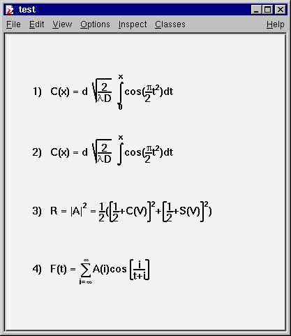
The picture generated by the tutorial macro latex.C
The script $ROOTSYS/tutorials/graphics/latex2.C:
{
  TCanvas c1("c1","Latex",600,700);
  TLatex l;
  l.SetTextAlign(23);
  l.SetTextSize(0.1);
  l.DrawLatex(0.5,0.95,"e^{+}e^{-}#rightarrowZ^{0}
  #rightarrowI#bar{I}, q#bar{q}");
  l.DrawLatex(0.5,0.75,"|#vec{a}#bullet#vec{b}|=
  #Sigmaa^{i}_{jk}+b^{bj}_{i}");
  l.DrawLatex(0.5,0.5,"i(#partial_{#mu}#bar{#psi}#gamma^{#mu}
  +m#bar{#psi}=0
  #Leftrightarrow(#Box+m^{2})#psi=0");
  l.DrawLatex(0.5,0.3,"L_{em}=eJ^{#mu}_{em}A_{#mu} ,
  J^{#mu}_{em}=#bar{I}#gamma_{#mu}I
  M^{j}_{i}=#SigmaA_{#alpha}#tau^{#alphaj}_{i}");
}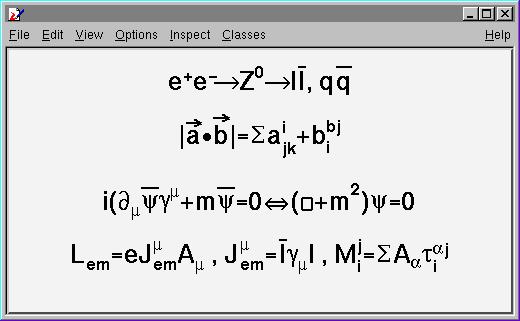
The picture generated by the tutorial macro latex2.C
The script $ROOTSYS/tutorials/graphics/latex3.C:
{
  TCanvas c1("c1");
  TPaveText pt(.1,.5,.9,.9);
  pt.AddText("#frac{2s}{#pi#alpha^{2}}
  #frac{d#sigma}{dcos#theta} (e^{+}e^{-}
  #rightarrow f#bar{f} ) = ");
  pt.AddText("#left| #frac{1}{1 - #Delta#alpha} #right|^{2}
  (1+cos^{2}#theta");
  pt.AddText("+ 4 Re #left{ #frac{2}{1 - #Delta#alpha} #chi(s)
  #[]{#hat{g}_{#nu}^{e}#hat{g}_{#nu}^{f}
  (1 + cos^{2}#theta) + 2 #hat{g}_{a}^{e}
  #hat{g}_{a}^{f} cos#theta) } #right}");
  pt.SetLabel("Born equation");
  pt.Draw();
}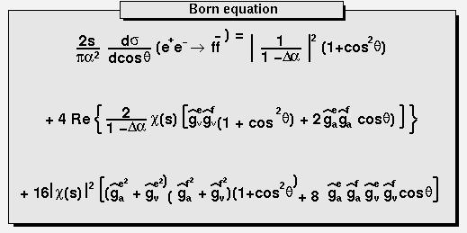
The picture generated by the tutorial macro latex3.C
Text displayed in a pad may be embedded into boxes, called paves, or may be drawn alone. In any case, it is recommended to use a Latex expression, which is covered in the previous paragraph. Using TLatex is valid whether the text is embedded or not. In fact, you will use Latex expressions without knowing it since it is the standard for all the embedded text. A pave is just a box with a border size and a shadow option. The options common to all types of paves and used when building those objects are the following:
option = "T" top frame
option = "B" bottom frame
option = "R" right frame
option = "L" left frame
option = "NDC" x1,y1,x2,y2 are given in NDC
option = "ARC" corners are rounded
We will see the practical use of these options in the description of the more functional objects like TPaveLabels. There are several categories of paves containing text: TPaveLabel, TPaveText and TPavesText. TPaveLabels are panels containing one line of text. They are used for labeling.
TPaveLabel(Double_t x1, Double_t y1, Double_t x2, Double_t y2,
           const char *label, Option_t *option)
Where (x1, y1) are the coordinates of the bottom left corner, (x2,y2) - coordinates of the upper right corner. “label” is the text to be displayed and “option” is the drawing option, described above. By default, the border size is 5 and the option is “br”. If one wants to set the border size to some other value, one may use the method SetBorderSize(). For example, suppose we have a histogram, which limits are (-100,100) in the x direction and (0, 1000) in the y direction. The following lines will draw a label in the center of the histogram, with no border. If one wants the label position to be independent of the histogram coordinates, or user coordinates, one can use the option “NDC”. See “The Coordinate Systems of a Pad”.
root[] pl = new TPaveLabel(-50,0,50,200,"Some text")
root[] pl->SetBorderSize(0)
root[] pl->Draw()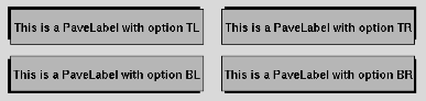
PaveLabels drawn with different options
A TPaveLabel can contain only one line of text. A TPaveText may contain several lines. This is the only difference. This picture illustrates and explains some of the points of TPaveText. Once a TPaveText is drawn, a line can be added or removed by brining up the context menu with the mouse.
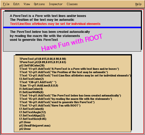
PaveText examples
A TPavesText is a stack of text panels (see TPaveText). One can set the number of stacked panels at building time. It has the following constructor: By default, the number of stacked panels is 5, option=“br”.
TPavesText(Double_t x1, Double_t y1, Double_t x2, Double_t y2,
Int_t npaves, Option_t* option)
A PaveText example
TMathText’s purpose is to write mathematical equations, exactly as TeX would do it. The syntax is the same as the TeX’s one.
The script $ROOTSYS/tutorials/graphics/tmathtex.C:
gives the following output:

A TMathText example
TMathText uses plain TeX syntax and uses “\” as control instead of “#”. If a piece of text containing “\” is given to TLatex then TMathText is automatically invoked. Therefore, as histograms’ titles, axis titles, labels etc … are drawn using TLatex, the TMathText syntax can be used for them also.
The axis objects are automatically built by various high level objects such as histograms or graphs. Once build, one may access them and change their characteristics. It is also possible, for some particular purposes to build axis on their own. This may be useful for example in the case one wants to draw two axis for the same plot, one on the left and one on the right.
For historical reasons, there are two classes representing axis. TAxis * axis is the axis object, which will be returned when calling the TH1::GetAxis() method.
TAxis *axis = histo->GetXaxis()Of course, you may do the same for Y and Z-axis. The graphical representation of an axis is done with the TGaxis class. The histogram classes and TGraph generate instances of this class. This is internal and the user should not have to see it.
The axis title is set, as with all named objects, by
axis->SetTitle("Whatever title you want");When the axis is embedded into a histogram or a graph, one has to first extract the axis object:
h->GetXaxis()->SetTitle("Whatever title you want")The axis options are most simply set with the styles. The available style options controlling specific axis options are the following:
TAxis *axis = histo->GetXaxis();
axis->SetAxisColor(Color_t color = 1);
axis->SetLabelColor(Color_t color = 1);
axis->SetLabelFont(Style_t font = 62);
axis->SetLabelOffset(Float_t offset = 0.005);
axis->SetLabelSize(Float_t size = 0.04);
axis->SetNdivisions(Int_t n = 510, Bool_t optim = kTRUE);
axis->SetNoExponent(Bool_t noExponent = kTRUE);
axis->SetTickLength(Float_t length = 0.03);
axis->SetTitleOffset(Float_t offset = 1);
axis->SetTitleSize(Float_t size = 0.02);
The getters corresponding to the described setters are also available. The general options, not specific to axis, as for instance SetTitleTextColor() are valid and do have an effect on axis characteristics.
Use TAxis::SetNdivisions(ndiv,optim) to set the number of divisions for an axis. The ndiv and optim are as follows:
ndiv = N1 + 100*N2 + 10000*N3
N1 = number of first divisions.
N2 = number of secondary divisions.
N3 = number of tertiary divisions.
optim = kTRUE (default), the divisions’ number will be optimized around the specified value.
optim = kFALSE, or n < 0, the axis will be forced to use exactly n divisions.
For example:
ndiv = 0: no tick marks.
ndiv = 2: 2 divisions, one tick mark in the middle of the axis.
ndiv = 510: 10 primary divisions, 5 secondary divisions
ndiv = -10: exactly 10 primary divisions
You can use TAxis::SetRange or TAxis::SetRangeUser to zoom the axis.
TAxis::SetRange(Int_t binfirst,Int_t binlast)The SetRange method parameters are bin numbers. They are not axis. For example if a histogram plots the values from 0 to 500 and has 100 bins, SetRange(0,10) will cover the values 0 to 50. The parameters for SetRangeUser are user coordinates. If the start or end is in the middle of a bin the resulting range is approximation. It finds the low edge bin for the start and the high edge bin for the high.
TAxis::SetRangeUser(Axis_t ufirst,Axis_t ulast)Both methods, SetRange and SetRangeUser, are in the context menu of any axis and can be used interactively. In addition, you can zoom an axis interactively: click on the axis on the start, drag the cursor to the end, and release the mouse button.
An axis may be drawn independently of a histogram or a graph. This may be useful to draw for example a supplementary axis for a graph. In this case, one has to use the TGaxis class, the graphical representation of an axis. One may use the standard constructor for this kind of objects:
TGaxis(Double_t xmin, Double_t ymin, Double_t xmax, Double_t ymax,
       Double_t wmin, Double_t wmax, Int_t ndiv = 510,
       Option_t* chopt,Double_t gridlength = 0)
The arguments xmin, ymin are the coordinates of the axis’ start in the user coordinates system, and xmax, ymax are the end coordinates. The arguments wmin and wmax are the minimum (at the start) and maximum (at the end) values to be represented on the axis; ndiv is the number of divisions. The options, given by the “chopt” string are the following:
chopt = 'G': logarithmic scale, default is linear.
chopt = 'B': Blank axis (it is useful to superpose the axis).
Instead of the wmin,wmax arguments of the normal constructor, i.e. the limits of the axis, the name of a TF1 function can be specified. This function will be used to map the user coordinates to the axis values and ticks.
The constructor is the following:
TGaxis(Double_t xmin, Double_t ymin, Double_t xmax, Double_t ymax,
       const char* funcname, Int_t ndiv=510,
       Option_t* chopt, Double_t gridlength=0)
In such a way, it is possible to obtain exponential evolution of the tick marks position, or even decreasing. In fact, anything you like.
Tick marks are normally drawn on the positive side of the axis, however, if xmin = xmax, then negative.
chopt = '+': tick marks are drawn on Positive side. (Default)
chopt = '-': tick marks are drawn on the negative side.
chopt = '+-': tick marks are drawn on both sides of the axis.
chopt = ‘U': unlabeled axis, default is labeled.
Labels are normally drawn on side opposite to tick marks. However, chopt = '=': on Equal side. The function TAxis::CenterLabels() sets the bit kCenterLabels and it is visible from TAxis context menu. It centers the bin labels and it makes sense only when the number of bins is equal to the number of tick marks. The class responsible for drawing the axis TGaxis inherits this property.
Labels are normally drawn parallel to the axis. However, if xmin = xmax, then they are drawn orthogonal, and if ymin=ymax they are drawn parallel.
By default, an exponent of the form 10^N is used when the label values are either all very small or very large. One can disable the exponent by calling:
TAxis::SetNoExponent(kTRUE)Note that this option is implicitly selected if the number of digits to draw a label is less than the fgMaxDigits global member. If the property SetNoExponent was set in TAxis (via TAxis::SetNoExponent), the TGaxis will inherit this property. TGaxis is the class responsible for drawing the axis. The method SetNoExponent is also available from the axis context menu.
Y-axis with and without exponent labels
TGaxis::fgMaxDigits is the maximum number of digits permitted for the axis labels above which the notation with 10^N is used. It must be greater than 0. By default fgMaxDigits is 5 and to change it use the TGaxis::SetMaxDigits method. For example to set fgMaxDigits to accept 6 digits and accept numbers like 900000 on an axis call:
TGaxis::SetMaxDigits(6)Labels are centered on tick marks. However, if xmin = xmax, then they are right adjusted.
chopt = 'R': labels are right adjusted on tick mark (default is centered)
chopt = 'L': labels are left adjusted on tick mark.
chopt = 'C': labels are centered on tick mark.
chopt = 'M': In the Middle of the divisions.
Blank characters are stripped, and then the label is correctly aligned. The dot, if last character of the string, is also stripped. In the following, we have some parameters, like tick marks length and characters height (in percentage of the length of the axis, in user coordinates). The default values are as follows:
Primary tick marks: 3.0 %
Secondary tick marks: 1.5 %
Third order tick marks: .75 %
Characters height for labels: 4%
Labels offset: 1.0 %
Use the TStyle::SetStripDecimals to strip decimals when drawing axis labels. By default, the option is set to true, and TGaxis::PaintAxis removes trailing zeros after the dot in the axis labels, e.g. {0, 0.5, 1, 1.5, 2, 2.5, etc.}
TStyle::SetStripDecimals (Bool_t strip=kTRUE)If this function is called with strip=kFALSE, TGaxis::PaintAxis() will draw labels with the same number of digits after the dot, e.g. {0.0, 0.5, 1.0, 1.5, 2.0, 2.5, etc.}
chopt = 'W': cross-Wire
By default, the axis binning is optimized.
chopt = 'N': No binning optimization
chopt = 'I': Integer labeling
Histograms’ axis can be defined as “time axis”. To do that it is enough to activate the SetTimeDisplay attribute on a given axis. If h is a histogram, it is done the following way:
h->GetXaxis()->SetTimeDisplay(1); // X axis is a time axisTwo parameters can be adjusted in order to define time axis: the time format and the time offset.
It defines the format of the labels along the time axis. It can be changed using the TAxis method SetTimeFormat. The time format is the one used by the C function strftime(). It is a string containing the following formatting characters:
For the date: |
%a abbreviated weekday name %b abbreviated month name %d day of the month (01-31) %m month (01-12) %y year without century %Y year with century |
For the time: |
%H hour (24-hour clock) %I hour (12-hour clock) %p local equivalent of AM or PM %M minute (00-59) %S seconds (00-61) %% % |
The other characters are output as is. For example to have a format like dd/mm/yyyy one should do:
h->GetXaxis()->SetTimeFormat("%d/%m/%Y");If the time format is not defined, a default one will be computed automatically.
This is a time in seconds in the UNIX standard UTC format (the universal time, not the local one), defining the starting date of a histogram axis. This date should be greater than 01/01/95 and is given in seconds. There are three ways to define the time offset:
1- By setting the global default time offset:
TDatime da(2003,02,28,12,00,00);
gStyle->SetTimeOffset(da.Convert());
If no time offset is defined for a particular axis, the default time offset will be used. In the example above, notice the usage of TDatime to translate an explicit date into the time in seconds required by SetTimeFormat.
2- By setting a time offset to a particular axis:
TDatime dh(2001,09,23,15,00,00);
h->GetXaxis()->SetTimeOffset(dh.Convert());
3- Together with the time format using SetTimeFormat. The time offset can be specified using the control character %F after the normal time format. %F is followed by the date in the format: yyyy-mm-dd hh:mm:ss.
h->GetXaxis()->SetTimeFormat("%d/%m/%y%F2000-02-28 13:00:01");Notice that this date format is the same used by the TDatime function AsSQLString. If needed, this function can be used to translate a time in seconds into a character string which can be appended after %F. If the time format is not specified (before %F) the automatic one will be used. The following example illustrates the various possibilities.
{
  gStyle->SetTitleH(0.08);
  TDatime da(2003,02,28,12,00,00);
  gStyle->SetTimeOffset(da.Convert());
  ct = new TCanvas("ct","Time on axis",0,0,600,600);
  ct->Divide(1,3);
  ht1 = new TH1F("ht1","ht1",30000,0.,200000.);
  ht2 = new TH1F("ht2","ht2",30000,0.,200000.);
  ht3 = new TH1F("ht3","ht3",30000,0.,200000.);
  for (Int_t i=1;i<30000;i++) {
    Float_t noise = gRandom->Gaus(0,120);
    ht1->SetBinContent(i,noise);
    ht2->SetBinContent(i,noise*noise);
    ht3->SetBinContent(i,noise*noise*noise);
  }
  ct->cd(1);
  ht1->GetXaxis()->SetLabelSize(0.06);
  ht1->GetXaxis()->SetTimeDisplay(1);
  ht1->GetXaxis()->SetTimeFormat("%d/%m/%y%F2000-02-2813:00:01");
  ht1->Draw();
  ct->cd(2);
  ht2->GetXaxis()->SetLabelSize(0.06);
  ht2->GetXaxis()->SetTimeDisplay(1);
  ht2->GetXaxis()->SetTimeFormat("%d/%m/%y");
  ht2->Draw();
  ct->cd(3);
  ht3->GetXaxis()->SetLabelSize(0.06);
  TDatime dh(2001,09,23,15,00,00);
  ht3->GetXaxis()->SetTimeDisplay(1);
  ht3->GetXaxis()->SetTimeOffset(dh.Convert());
  ht3->Draw();
}
The output is shown in the figure below. If a time axis has no specified time offset, the global time offset will be stored in the axis data structure. The histogram limits are in seconds. If wmin and wmax are the histogram limits, the time axis will spread around the time offset value from TimeOffset+wmin to TimeOffset+wmax. Until now all examples had a lowest value equal to 0. The following example demonstrates how to define the histogram limits relatively to the time offset value.
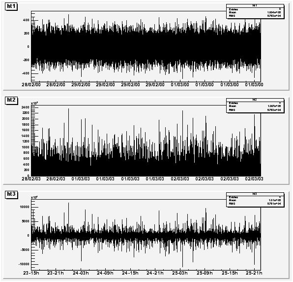
Time axis examples
{
  // Define the time offset as 2003, January 1st
  TDatime T0(2003,01,01,00,00,00);
  int X0 = T0.Convert();
  gStyle->SetTimeOffset(X0);

  // Define the lowest histogram limit as 2002,September 23rd
   TDatime T1(2002,09,23,00,00,00);
   int X1 = T1.Convert()-X0;

  // Define the highest histogram limit as 2003, March 7th
  TDatime T2(2003,03,07,00,00,00);
  int X2 = T2.Convert(1)-X0;

  TH1F * h1 = new TH1F("h1","test",100,X1,X2);

  TRandom r;
  for (Int_t i=0;i<30000;i++) {
    Double_t noise = r.Gaus(0.5*(X1+X2),0.1*(X2-X1));
    h1->Fill(noise);
  }

  h1->GetXaxis()->SetTimeDisplay(1);
  h1->GetXaxis()->SetLabelSize(0.03);
  h1->GetXaxis()->SetTimeFormat("%Y/%m/%d");
  h1->Draw();
}
The output is shown in the next figure. Usually time axes are created automatically via histograms, but one may also want to draw a time axis outside a “histogram context”. Therefore, it is useful to understand how TGaxis works for such axis. The time offset can be defined using one of the three methods described before. The time axis will spread around the time offset value. Actually, it will go from TimeOffset+wmin to TimeOffset+wmax where wmin and wmax are the minimum and maximum values (in seconds) of the axis. Let us take again an example. Having defined “2003, February 28 at 12h”, we would like to see the axis a day before and a day after.
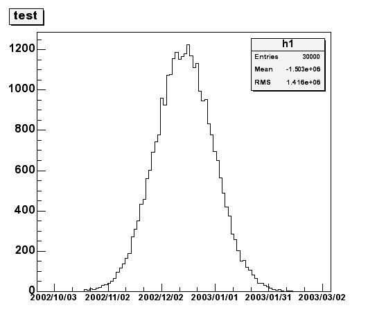
A histogram with time axis X
A TGaxis can be created the following way (a day has 86400 seconds):
TGaxis *axis = new TGaxis(x1,y1,x2,y2,-100000,150000,2405,"t");the “t” option (in lower case) means it is a “time axis”. The axis goes form 100000 seconds before TimeOffset and 150000 seconds after. So the complete macro is:
{
  c1 = new TCanvas("c1","Examples of TGaxis",10,10,700,500);
  c1->Range(-10,-1,10,1);
  TGaxis *axis = new TGaxis(-8,-0.6,8,-0.6,-100000,150000,2405,"t");
  axis->SetLabelSize(0.03);

  TDatime da(2003,02,28,12,00,00);
  axis->SetTimeOffset(da.Convert());
  axis->SetTimeFormat("%d/%m/%Y");
  axis->Draw();
}
The time format is specified with:
axis->SetTimeFormat("%d/%m/%Y");The macro gives the following output:
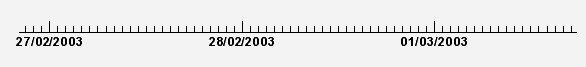
Thanks to the TLatex directive #splitline it is possible to write the time labels on two lines. In the previous example changing the SetTimeFormat line by:
axis->SetLabelOffset(0.02);
axis->SetTimeFormat("#splitline{%Y}{%d/%m}");
will produce the following axis:

To illustrate what was said, we provide two scripts. The first one creates the picture shown in the next figure.
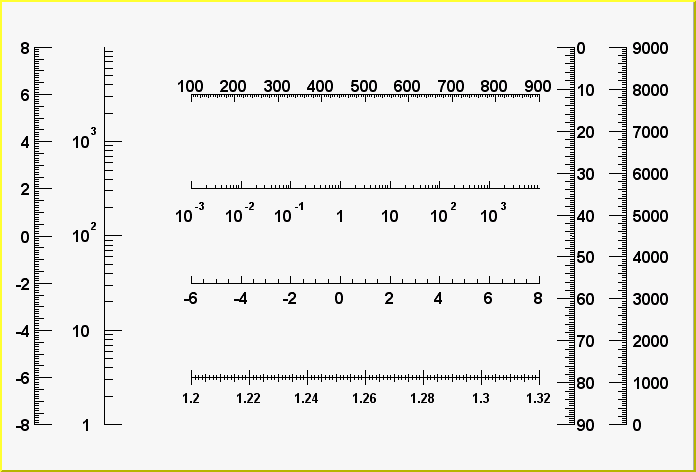
The first axis example
The first script is:
{
  c1 = new TCanvas("c1","Examples of Gaxis",10,10,700,500);
  c1->Range(-10,-1,10,1);

  TGaxis *axis1 = new TGaxis(-4.5,-0.2,5.5,-0.2,-6,8,510,"");
  axis1->SetName("axis1");
  axis1->Draw();
  TGaxis *axis2 = new TGaxis(4.5,0.2,5.5,0.2,0.001,10000,510,"G");
  axis2->SetName("axis2");
  axis2->Draw();

  TGaxis *axis3 = new TGaxis(-9,-0.8,-9,0.8,-8,8,50510,"");
  axis3->SetName("axis3");
  axis3->Draw();
  TGaxis *axis4 = new TGaxis(-7,-0.8,7,0.8,1,10000,50510,"G");
  axis4->SetName("axis4");
  axis4->Draw();

  TGaxis *axis5 = new TGaxis(-4.5,-6,5.5,-6,1.2,1.32,80506,"-+");
  axis5->SetName("axis5");
  axis5->SetLabelSize(0.03);
  axis5->SetTextFont(72);
  axis5->SetLabelOffset(0.025);
  axis5->Draw();

  TGaxis *axis6 = new TGaxis(-4.5,0.6,5.5,0.6,100,900,50510,"-");
  axis6->SetName("axis6");
  axis6->Draw();
  TGaxis *axis7 = new TGaxis(8,-0.8,8,0.8,0,9000,50510,"+L");
  axis7->SetName("axis7");
  axis7->SetLabelOffset(0.01);
  axis7->Draw();

  // one can make axis top->bottom. However because of a problem,
  // the two x values should not be equal
  TGaxis *axis8 = new TGaxis(6.5,0.8,6.499,-0.8,0,90,50510,"-");
  axis8->SetName("axis8");
  axis8->Draw();
}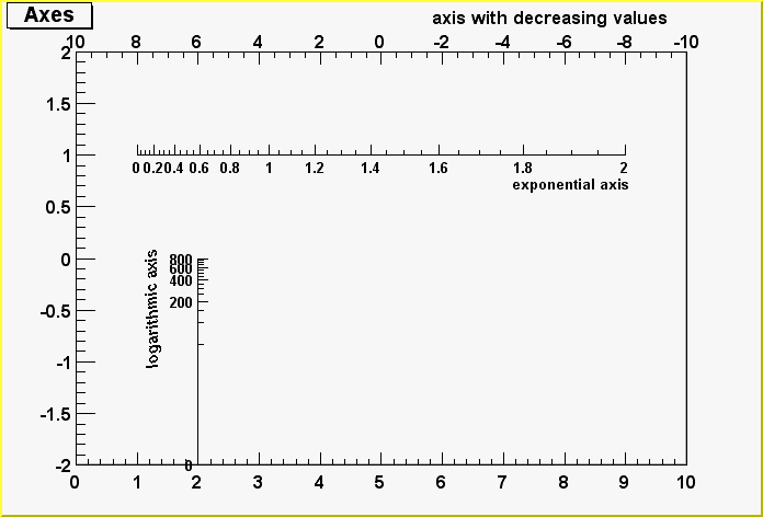
The second axis example
The second example shows the use of the second form of the constructor, with axis ticks position determined by a function TF1:
void gaxis3a()
{
  gStyle->SetOptStat(0);

  TH2F *h2 = new TH2F("h","Axes",2,0,10,2,-2,2);
  h2->Draw();
  TF1 *f1=new TF1("f1","-x",-10,10);
  TGaxis *A1 = new TGaxis(0,2,10,2,"f1",510,"-");
  A1->SetTitle("axis with decreasing values");
  A1->Draw();

  TF1 *f2=new TF1("f2","exp(x)",0,2);
  TGaxis *A2 = new TGaxis(1,1,9,1,"f2");
  A2->SetTitle("exponential axis");
  A2->SetLabelSize(0.03);
  A2->SetTitleSize(0.03);
  A2->SetTitleOffset(1.2);
  A2->Draw();

  TF1 *f3=new TF1("f3","log10(x)",0,800);
  TGaxis *A3 = new TGaxis(2,-2,2,0,"f3",505);
  A3->SetTitle("logarithmic axis");
  A3->SetLabelSize(0.03);
  A3->SetTitleSize(0.03);
  A3->SetTitleOffset(1.2);
  A3->Draw();
}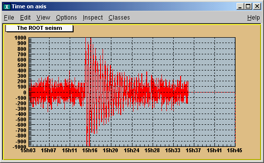
An axis example with time display
// strip chart example
void seism() {

  TStopwatch sw; sw.Start();
  //set time offset
  TDatime dtime;
  gStyle->SetTimeOffset(dtime.Convert());
  TCanvas *c1 = new TCanvas("c1","Time on axis",10,10,1000,500);
  c1->SetFillColor(42);
  c1->SetFrameFillColor(33);
  c1->SetGrid();

  Float_t bintime = 1;
  // one bin = 1 second. change it to set the time scale
  TH1F *ht = new TH1F("ht","The ROOT seism",10,0,10*bintime);
  Float_t signal = 1000;
  ht->SetMaximum(signal);
  ht->SetMinimum(-signal);
  ht->SetStats(0);
  ht->SetLineColor(2);
  ht->GetXaxis()->SetTimeDisplay(1);
  ht->GetYaxis()->SetNdivisions(520);
  ht->Draw();

  for (Int_t i=1;i<2300;i++) {
    // Build a signal : noisy damped sine
    Float_t noise  = gRandom->Gaus(0,120);
    if (i > 700)
      noise += signal*sin((i-700.)*6.28/30)*exp((700.-i)/300.);
    ht->SetBinContent(i,noise);
    c1->Modified();
    c1->Update();
    gSystem->ProcessEvents();
    //canvas can be edited during the loop
   }
   printf("Real Time = %8.3fs,Cpu Time = %8.3fsn",sw.RealTime(),
          sw.CpuTime());
}When a class contains text or derives from a text class, it needs to be able to set text attributes like font type, size, and color. To do so, the class inherits from the TAttText class (a secondary inheritance), which defines text attributes. TLatex and TText inherit from TAttText.
Text alignment may be set by a method call. What is said here applies to all objects deriving from TAttText, and there are many. We will take an example that may be transposed to other types. Suppose “la” is a TLatex object. The alignment is set with:
root[] la->SetTextAlign(align)The parameter align is a short describing the alignment:
align = 10*HorizontalAlign + VerticalAlign
For horizontal alignment, the following convention applies:
1 = left
2 = centered
3 = right
For vertical alignment, the following convention applies:
1 = bottom
2 = centered
3 = top
For example, align: 11 = left adjusted and bottom adjusted; 32 = right adjusted and vertically centered.
Use TAttText::SetTextAngle to set the text angle. The angle is the degrees of the horizontal.
root[] la->SetTextAngle(angle)Use TAttText::SetTextColor to set the text color. The color is the color index. The colors are described in “Color and Color Palettes”.
root[] la->SetTextColor(color)Use TAttText::SetTextFont to set the font. The parameter font is the font code, combining the font and precision: font = 10 * fontID + precision
root[] la->SetTextFont(font)The table below lists the available fonts. The font IDs must be between 1 and 14. The precision can be:
Precision = 0 fast hardware fonts (steps in the size)
Precision = 1 scalable and rotate-able hardware fonts (see below)
Precision = 2 scalable and rotate-able hardware fonts
When precision 0 is used, only the original non-scaled system fonts are used. The fonts have a minimum (4) and maximum (37) size in pixels. These fonts are fast and are of good quality. Their size varies with large steps and they cannot be rotated. Precision 1 and 2 fonts have a different behavior depending if True Type Fonts (TTF) are used or not. If TTF are used, you always get very good quality scalable and rotate-able fonts. However, TTF are slow. Precision 1 and 2 fonts have a different behavior for PostScript in case of TLatex objects:
With precision 1, the PostScript text uses the old convention (see TPostScript) for some special characters to draw sub and superscripts or Greek text.
With precision 2, the “PostScript” special characters are drawn as such. To draw sub and superscripts it is highly recommended to use TLatex objects instead.
For example: font = 62 is the font with ID 6 and precision 2.
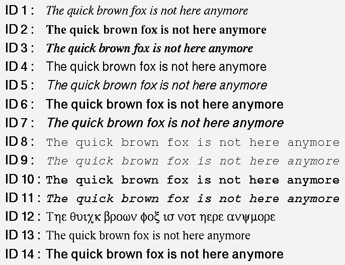
Font’s examples
The available fonts are:
Font ID |
X11 |
True Type name |
Is italic |
“boldness” |
1 |
times-medium-i-normal |
“Times New Roman” |
Yes |
4 |
2 |
times-bold-r-normal |
“Times New Roman” |
No |
7 |
3 |
times-bold-i-normal |
“Times New Roman” |
Yes |
7 |
4 |
helvetica-medium-r-norma l |
“Arial” |
No |
4 |
5 |
helvetica-medium-o-norma l |
“Arial” |
Yes |
4 |
6 |
helvetica-bold-r-normal |
“Arial” |
No |
7 |
7 |
helvetica-bold-o-normal |
“Arial” |
Yes |
7 |
8 |
courier-medium-r-normal |
“Courier New” |
No |
4 |
9 |
courier-medium-o-normal |
“Courier New” |
Yes |
4 |
10 |
courier-bold-r-normal |
“Courier New” |
No |
7 |
11 |
courier-bold-o-normal |
“Courier New” |
Yes |
7 |
12 |
symbol-medium-r-normal |
“Symbol” |
No |
6 |
13 |
times-medium-r-normal |
“Times New Roman” |
No |
4 |
14 |
“Wingdings” |
No |
4 |
This script makes the image of the different fonts:
{
  textc = new TCanvas("textc","Example of text",1);
  for (int i=1;i<15;i++) {
    cid = new char[8];
    sprintf(cid,"ID %d :",i);
    cid[7] = 0;
    lid = new TLatex(0.1,1-(double)i/15,cid);
    lid->SetTextFont(62);
    lid->Draw();
    l = new TLatex(.2,1-(double)i/15,
                   "The quick brown fox is not here anymore")
    l->SetTextFont(i*10+2);
    l->Draw();
  }
}You can activate the True Type Fonts by adding the following line in your .rootrc file.
Unix.*.Root.UseTTFonts: trueYou can check that you indeed use the TTF in your Root session. When the TTF is active, you get the following message at the start of a session: “Free Type Engine v1.x used to render TrueType fonts.” You can also check with the command:
gEnv->Print()Use TAttText::SetTextSize to set the text size.
root[] la->SetTextSize(size)The size is the text size expressed in percentage of the current pad size.
The text size in pixels will be:
If current pad is horizontal, the size in pixels = textsize * canvas_height
If current pad is vertical, the size in pixels = textsize * canvas_width
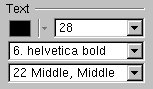 The user interface for changing the text color, size, font and allignment looks like shown in this picture. It takes place in the editor frame anytime the selected object inherits the class
 TAttText.
All classes manipulating lines have to deal with line attributes: color, style and width. This is done by using secondary inheritance of the class TAttLine. The line color may be set by a method call. What is said here applies to all objects deriving from TAttLine, and there are many (histograms, plots). We will take an example that may be transposed to other types. Suppose “li” is a TLine object. The line color is set with:
root[] li->SetLineColor(color)The argument color is a color number. The colors are described in “Color and Color Palettes”
The line style may be set by a method call. What is said here applies to all objects deriving from TAttLine, and there are many (histograms, plots). We will take an example that may be transposed to other types. Suppose “li” is a TLine object. The line style is set with:
root[] li->SetLineStyle(style)The argument style is one of: 1=solid, 2=dash, 3=dot, 4=dash-dot.
The line width may be set by a method call. What is said here applies to all objects deriving from TAttLine, and there are many (histograms, plots). We will take an example that may be transposed to other types. Suppose “li” is a TLine object. The line width is set with:
root[] li->SetLineWidth(width)The width is the width expressed in pixel units.
 The user interface for changing the line color, line width and style looks like shown in this picture. It takes place in the editor frame anytime the selected object inherits the class
 TAttLine.
Almost all graphics classes have a fill area somewhere. These classes have to deal with fill attributes. This is done by using secondary inheritance of the class TAttFill. Fill color may be set by a method call. What is said here applies to all objects deriving from TAttFill, and there are many (histograms, plots). We will take an example that may be transposed to other types. Suppose “h” is a TH1F (1 dim histogram) object. The histogram fill color is set with:
root[] h->SetFillColor(color)The color is a color number. The colors are described in “Color and color palettes”
Fill style may be set by a method call. What is said here applies to all objects deriving from TAttFill, and there are many (histograms, plots). We will take an example that may be transposed to other types. Suppose “h” is a TH1F (1 dim histogram) object. The histogram fill style is set with:
root[] h->SetFillStyle(style)The convention for style is: 0:hollow, 1001:solid, 2001:hatch style, 3000+pattern number:patterns, 4000 to 4100:transparency, 4000:fully transparent, 4100: fully opaque.
Fill styles >3100 and <3999 are hatches. They are defined according to the FillStyle=3ijk value as follows:
i(1-9) specifies the space between each hatch (1=minimum space, 9=maximum). The final spacing is set by SetHatchesSpacing() method and it is*GetHatchesSpacing().
j(0-9) specifies the angle between 0 and 90 degres as follows: 0=0, 1=10, 2=20, 3=30, 4=45, 5=not drawn, 6=60, 7=70, 8=80 and 9=90.
k(0-9) specifies the angle between 0 and 90 degres as follows: 0=180, 1=170, 2=160, 3=150, 4=135, 5=not drawn, 6=120, 7=110, 8=100 and 9=90.
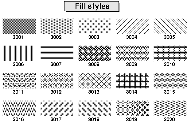
The various patterns
At initialization time, a table of basic colors is generated when the first Canvas constructor is called. This table is a linked list, which can be accessed from the gROOT object (see TROOT::GetListOfColors()). Each color has an index and when a basic color is defined, two “companion” colors are defined:
the dark version (color index + 100)
the bright version (color index + 150)
The dark and bright colors are used to give 3-D effects when drawing various boxes (see TWbox, TPave, TPaveText, TPaveLabel, etc). If you have a black and white copy of the manual, here are the basic colors and their indices.
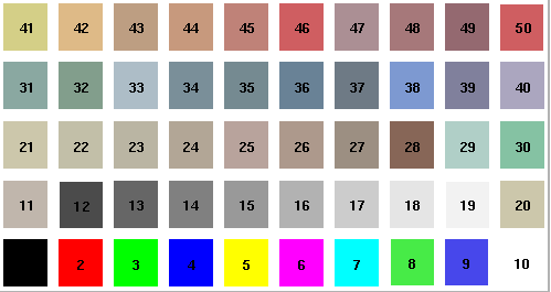
The basic ROOT colors

The list of currently supported basic colors (here dark and bright colors are not shown) are shown. The color numbers specified in the basic palette, and the picture above, can be viewed by selecting the menu entry Colors in the View canvas menu. The user may define other colors. To do this, one has to build a new TColor:
TColor(Int_t color,Float_t r,Float_t g,Float_t b,const char* name)One has to give the color number and the three Red, Green, Blue values, each being defined from 0 (min) to 1(max). An optional name may be given. When built, this color is automatically added to the existing list of colors. If the color number already exists, one has to extract it from the list and redefine the RGB values. This may be done for example with:
root[] color=(TColor*)(gROOT->GetListOfColors()->At(index_color))
root[] color->SetRGB(r,g,b)
Where r, g and b go from 0 to 1 and index_color is the color number you wish to change.
 The user interface for changing the fill color and style looks like shown in this picture. It takes place in the editor frame anytime the selected object inherits the class
 TAttFill.
Defining one color at a time may be tedious. The histogram classes (see Draw Options) use the color palette. For example, TH1::Draw("col") draws a 2-D histogram with cells represented by a box filled with a color CI function of the cell content. If the cell content is N, the color CI used will be the color number in colors[N]. If the maximum cell content is >ncolors, all cell contents are scaled to ncolors. The current color palette does not have a class or global object of its own. It is defined in the current style as an array of color numbers. The current palette can be changed with:
TStyle::SetPalette(Int_t ncolors,Int_t*color_indexes).By default, or if ncolors <= 0, a default palette (see above) of 50 colors is defined. The colors defined in this palette are good for coloring pads, labels, and other graphic objects. If ncolors > 0 and colors = 0, the default palette is used with a maximum of ncolors. If ncolors == 1 && colors == 0, then a pretty palette with a spectrum Violet->Red is created. It is recommended to use this pretty palette when drawing lego(s), surfaces or contours. For example, to set the current palette to the “pretty” one, do:
root[] gStyle->SetPalette(1)A more complete example is shown below. It illustrates the definition of a custom palette. You can adapt it to suit your needs. In case you use it for contour coloring, with the current color/contour algorithm, always define two more colors than the number of contours.
void palette() {
  // Example of creating new colors (purples)
  const Int_t colNum = 10;    // and defining of a new palette
  Int_t palette[colNum];
  for (Int_t i=0; i<colNum; i++) {
    // get the color and if it does not exist create it
    if (! gROOT->GetColor(230+i) ){
      TColor *color =
         new TColor(230+i,1-(i/((colNum)*1.0)),0.3,0.5,"");
    } else {
      TColor *color = gROOT->GetColor(230+i);
      color->SetRGB(1-(i/((colNum)*1.0)),0.3,0.5);
    }
    palette[i] = 230+i;
  }
  gStyle->SetPalette(colNum,palette);
  TF2 *f2 = new TF2("f2","exp(-(x^2)-(y^2))",-3,3,-3,3);
  // two contours less than the number of colors in palette
  f2->SetContour(colNum-2);
  f2->Draw("cont");
}A new graphics editor took place in ROOT v4.0. The editor can be activated by selecting the Editor menu entry in the canvas View menu or one of the context menu entries for setting line, fill, marker or text attributes. The following object editors are available for the current ROOT version.
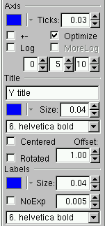
This user interface gives the possibility for changing the following axis attributes:
color of the selected axis, the axis’ title and labels;
the length of thick parameters and the possibility to set them on both axis sides (if +- is selected);
to set logarithmic or linear scale along the selected axis with a choice for optimized or more logarithmic labels;
primary, secondary and tertiary axis divisions can be set via the three number fields;
the axis title can be added or edited and the title’s color, position, offset, size and font can be set interactively;
the color, size, and offset of axis labels can be set similarly. In addition, there is a check box for no exponent choice, and another one for setting the same decimal part for all labels.
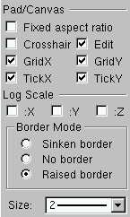
It provides the following user interface:
Fixed aspect ratio - can be set for pad resizing.
Edit - sets pad or canvas as editable.
Cross-hair - sets a cross hair on the pad.
TickX - set ticks along the X axis.
TickY - set ticks along the Y axis.
GridX - set a grid along the X axis.
GridY - set a grid along the Y axis.
The pad or canvas border size can be set if a sunken or a raised border mode is
selected; no border mode can be set too.
You can make a copy of a canvas using TCanvas::DrawClonePad. This method is unique to TCanvas. It clones the entire canvas to the active pad. There is a more general method TObject::DrawClone, which all objects descendent of TObject, specifically all graphic objects inherit. Below are two examples, one to show the use of DrawClonePad and the other to show the use of DrawClone.
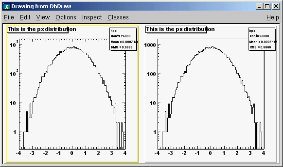
In this example we will copy an entire canvas to a new one with DrawClonePad. Run the script draw2dopt.C.
root[] .x tutorials/hist/draw2dopt.CThis creates a canvas with 2D histograms. To make a copy of the canvas follow the steps:
Right-click on it to bring up the context menu
Select DrawClonePad
This copies the entire canvas and all its sub-pads to a new canvas. The copied canvas is a deep clone, and all the objects on it are copies and independent of the original objects. For instance, change the fill on one of the original histograms, and the cloned histogram retains its attributes. DrawClonePad will copy the canvas to the active pad; the target does not have to be a canvas. It can also be a pad on a canvas.
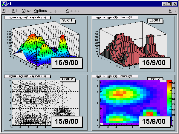
Different draw options
If you want to copy and paste a graphic object from one canvas or pad to another canvas or pad, you can do so with DrawClone method inherited from TObject. All graphics objects inherit the TObject::DrawClone method. In this example, we create a new canvas with one histogram from each of the canvases from the script draw2dopt.C.
Start a new ROOT session and execute the script draw2dopt.C
Select a canvas displayed by the script, and create a new canvas c1 from the File menu.
Make sure that the target canvas (c1) is the active one by middle clicking on it. If you do this step right after step 2, c1 will be active.
Select the pad with the first histogram you want to copy and paste.
Right click on it to show the context menu, and select DrawClone.
Leave the option blank and hit OK.
Repeat these steps for one histogram on each of the canvases created by the script, until you have one pad from each type. If you wanted to put the same annotation on each of the sub pads in the new canvas, you could use DrawClone to do so. Here we added the date to each pad. The steps to this are:
Create the label in on of the pads with the graphics editor.
Middle-click on the target pad to make it the active pad
Use DrawClone method of the label to draw it in each of the other panels.
The option in the DrawClone method argument is the Draw option for a histogram or graph. A call to TH1::DrawClone can clone the histogram with a different draw option.
To copy and paste the four pads from the command line or in a script you would execute the following statements:
root[] .x tutorials/hist/draw2dopt.C
root[] TCanvas c1("c1","Copy Paste",200,200,800,600);
root[] surfaces->cd(1); // get the first pad
root[] TPad *p1 = gPad;
root[] lego->cd(2);// get the next pad
root[] TPad *p2 = gPad;
root[] cont->cd(3);// get the next pad
root[] TPad *p3 = gPad;
root[] c2h->cd(4);// get the next pad
root[] TPad *p4 = gPad;
root[] // to draw the four clones
root[] c1->cd();
root[] p1->DrawClone();
root[] p2->DrawClone();
root[] p3->DrawClone();
root[] p4->DrawClone();
Note that the pad is copied to the new canvas in the same location as in the old canvas. For example if you were to copy the third pad of surf to the top left corner of the target canvas you would have to reset the coordinates of the cloned pad.
Legends for a graph are obtained with a TLegend object. This object points to markers, lines, boxes, histograms, graphs and represent their marker, line, fill attributes. Any object that has a marker or line or fill attribute may have an associated legend. A TLegend is a panel with several entries (class TLegendEntry) and is created by the constructor
TLegend(Double_t x1, Double_t y1, Double_t x2, Double_t y2,
        const char *header, Option_t *option)
The legend is defined with default coordinates, border size and option. The legend coordinates (NDC) in the current pad are x1, y1, x2, y2. The default text attributes for the legend are:
Alignment = 12 left adjusted and vertically centered
Angle = 0 (degrees)
Color = 1 (black)
Size = calculate when number of entries is known
Font = helvetica-medium-r-normal scalable font = 42, and bold = 62 for title
The title is a regular entry and supports TLatex. The default is no title (header = 0). The options are the same as for TPave; by default, they are “brand”. Once the legend box is created, one has to add the text with the AddEntry() method:
TLegendEntry* TLegend::AddEntry(TObject *obj,
                                const char *label,
                                Option_t *option)
The parameters are:
*objis a pointer to an object having marker, line, or fill attributes (a histogram, or a graph)
label is the label to be associated to the object
option:
“L” draw line associated with line attributes of obj, if obj inherits from TAttLine.
“P” draw poly-marker associated with marker attributes of obj, if obj inherits TAttMarker.
“F” draw a box with fill associated with fill attributes of obj, if obj inherits TAttFill.
One may also use the other form of the method AddEntry:
TLegendEntry* TLegend::AddEntry(const char *name,
                                const char *label,
                                Option_t *option)
Here name is the name of the object in the pad. Other parameters are as in the previous case. Next example shows how to create a legend:
leg = new TLegend(0.4,0.6,0.89,0.89);
leg->AddEntry(fun1,"One Theory","l");
leg->AddEntry(fun3,"Another Theory","f");
leg->AddEntry(gr,"The Data","p");
leg->Draw();
// oops we forgot the blue line... add it after
leg->AddEntry(fun2,
              "#sqrt{2#pi} P_{T} (#gamma) latex  formula","f");
// and add a header (or "title") for the legend
leg->SetHeader("The Legend Title");
leg->Draw();
Here fun1, fun2, fun3 and gr are pre-existing functions and graphs. You can edit the TLegend by right clicking on it.
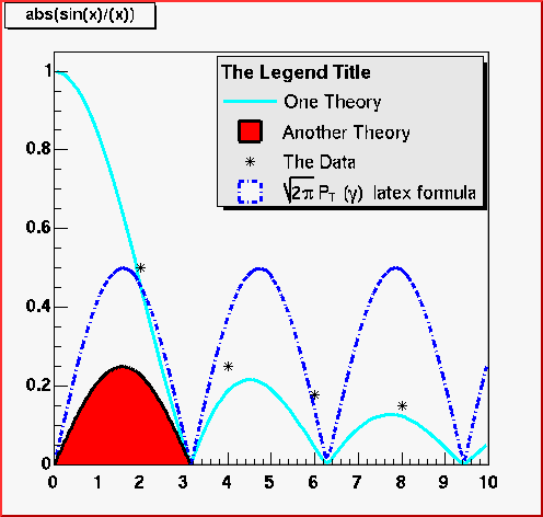
A legend example
To generate a PostScript (or encapsulated PostScript) file for a single image in a canvas, you can:
Select to print the canvas in the PostScript file format from the File menu / Save or Save As menu entries. By default, a PostScript file is generated, if you do not specify the file format.
Click in the canvas area, near the edges, with the right mouse button and select the Print context menu entry. This will generate a file of canvas pointed to by c1. You can select the name of the PostScript file. If the file name is xxx.ps, you will generate a PostScript file named xxx.ps. If the file name is xxx.eps, you generate an encapsulated Postscript file instead. In your program (or script), you can type:
c1->Print("xxx.ps") // or
c1->Print("xxx.eps")
Next example prints the picture in the pad pointed by pad1.
pad1->Print("xxx.ps")The TPad::Print method has a second parameter called option. Its value can be:
0 which is the default and is the same as “ps”
“ps” a Postscript file is produced
“Portrait” a Postscript file is produced with Portrait orientation
“Landscape” a Postscript file is produced with Landscape orientation
“eps”an Encapsulated Postscript file
“Preview”an Encapsulated Postscript file with preview is produced
“gif” a Graphics Interchange Format file
“cxx” a C++ macro file is generated
“pdf”a Portable Document Format file
“xml” a eXtensible Mark-up Language file
“jpg”a Joint Photographic Experts Group file
“png” a Portable Network Graphics Format (PNG file)
“xpm” a X11 Pixel Map Format
“svg” a Scalable Vector Graphics file
“tiff” a Tagged-Image File Format
“root”a ROOT binary file is produced
You do not need to specify this second parameter; you can indicate by the filename extension what format you want to save a canvas in (i.e. canvas.ps, canvas.gif, canvas.C, etc).
The size of the PostScript picture, by default, is computed to keep the aspect ratio of the picture on the screen, where the size along x is always 20 cm. You can set the size of the PostScript picture before generating the picture with a command such as:
TPostScript myps("myfile.ps",111)
myps.Range(xsize,ysize);
object->Draw();
myps.Close();
The first parameter in the TPostScript constructor is the name of the file; the second one is the format option:
111 - ps portrait
112 - ps landscape
113 - eps
You can set the default paper size with:
gStyle->SetPaperSize(xsize,ysize);You can resume writing again in this file with myps.Open(). Note that you may have several Post Script files opened simultaneously. Use TPostScript::Text(x,y,"string") to add text to a postscript file. This method writes the string in quotes into a PostScript file at position x, y in world coordinates.
The following characters have a special action on the PostScript file:
` - go to Greek
' - go to special
~ - go to Zapf Dingbats
? - go to subscript
^ - go to superscript
! - go to normal level of script
& - backspace one character
# - end of Greek or end of ZapfDingbats
These special characters are printed as such on the screen. To generate one of these characters on the PostScript file, you must escape it with the escape character “@”. The use of these special characters is illustrated in several scripts referenced by the TPostScript constructor.
The following sequence writes the canvas to “c1.ps” and closes the postscript file:
TCanvas c1("c1");
h1.Draw();
c1.Print("c1.ps");
If the Postscript file name finishes with “(”, the file remains opened (it is not closed). If the Postscript file name finishes with “)” and the file has been opened with “(”, the file is closed.
{
   TCanvas c1("c1");
   h1.Draw();
   c1.Print("c1.ps("); // write canvas and keep the ps file open
   h2.Draw();
   c1.Print("c1.ps");  // canvas is added to "c1.ps"
   h3.Draw();
   c1.Print("c1.ps)"); // canvas is added to "c1.ps"
                       // and ps file is closed
}
The TCanvas::Print("file.ps(") mechanism is very useful, but it can be a little inconvenient to have the action of opening/closing a file being atomic with printing a page. Particularly if pages are being generated in some loop, one needs to detect the special cases of first and last page. The “[” and “]” can be used instead of “(” and “)” as shown in the next example.
c1.Print("file.ps[");      // no actual print; just open file.ps
for (i=0; i<10; ++i) {
   // fill canvas for context i
   ...
   c1.Print("file.ps");   // actually print canvas to file.ps
}  // end loop
c1.Print("file.ps]");     // no actual print; just close file.ps
The following script illustrates how to open a postscript file and draw several pictures. The generation of a new postscript page is automatic when TCanvas::Clear is called by object->Draw().
{
   TFile f("hsimple.root");
   TCanvas c1("c1","canvas",800,600);

   //select PostScript  output type
   Int_t type = 111;         //portrait  ps
   // Int_t type = 112;      //landscape ps
   // Int_t type = 113;      //eps

   //create a PostScript  file and set the paper size
   TPostScript ps("test.ps",type);
   ps.Range(16,24);          //set x,y of printed page

   //draw 3 histograms from file hsimple.root on separate pages
   hpx->Draw();
   c1.Update();              //force drawing in a script
   hprof->Draw();
   c1.Update();
   hpx->Draw("lego1");
   c1.Update();
   ps.Close();
}
The next example does the same:
{
   TFile f("hsimple.root");
   TCanvas c1("c1","canvas",800,600);

   //set x,y of printed page
   gStyle->SetPaperSize(16,24);

   //draw 3 histograms from file hsimple.root on separate pages
   hpx->Draw();
   c1->Print("test1.ps(", "Portrait");
   hprof->Draw();
   c1->Print("test1.ps");
   hpx->Draw("lego1");
   c1->Print("test1.ps)");
}
This following example shows two pages. The canvas is divided. TPostScript::NewPage must be called before starting a new picture. object->Draw does not clear the canvas in this case because we clear only the pads and not the main canvas. Note that c1->Update must be called at the end of the first picture.
{
   TFile *f1 = new TFile("hsimple.root");
   TCanvas *c1 = new TCanvas("c1");
   TPostScript *ps = new TPostScript("file.ps",112);

   // picture 1
   c1->Divide(2,1);
   ps->NewPage();
   c1->cd(1);
   hpx->Draw();
   c1->cd(2);
   hprof->Draw();

   // picture 2
   c1->Update();
   ps->NewPage();
   c1->cd(1);
   hpxpy->Draw();
   c1->cd(2);
   ntuple->Draw("px");
   c1->Update();
   ps->Close();

   // invoke PostScript  viewer
   gSystem->Exec("gs file.ps");
}
The next one does the same:
{
   TFile *f1 = new TFile("hsimple.root");
   TCanvas *c1 = new TCanvas("c1");
   c1->Divide(2,1);

   // picture 1
   c1->cd(1);
   hpx->Draw();
   c1->cd(2);
   hprof->Draw();
   c1->Print("test2.ps(", "Landscape");

   // picture 2
   c1->cd(1);
   hpxpy->Draw();
   c1->cd(2);
   ntuple->Draw("px");
   c1->Print("test2.ps)");
   gSystem->Exec("gs file.ps");  // invoke PostScript  viewer
}TPostScript (and TPDF) support two color models: RGB and CMYK. CMY and CMYK models are subtractive color models unlike RGB which is an additive. They are mainly used for printing purposes. CMY means Cyan Magenta Yellow to convert RGB to CMY it is enough to do: C=1-R, M=1-G and Y=1-B. CMYK has one more component K (black). The conversion from RGB to CMYK is:
 Double_t Black   = TMath::Min(TMath::Min(1-Red,1-Green),1-Blue);
 Double_t Cyan    = (1-Red-Black)/(1-Black);
 Double_t Magenta = (1-Green-Black)/(1-Black);
 Double_t Yellow  = (1-Blue-Black)/(1-Black);
CMYK add the black component which allows to have a better quality for black printing. TPostScript (and TPDF) support the CMYK model. To change the color model use:
gStyle->SetColorModelPS(c);c = 0 means TPostScript will use RGB color model (default)c = 1 means TPostScript will use CMYK color modelLike PostScript, PDF is a vector graphics output format allowing a very high graphics output quality. The functionnalities provided by this class are very similar to those provided by TPostScript`.
Compare to PostScript output, the PDF files are usually smaller because some parts of them can be compressed.
PDF also allows to define table of contents. This facility can be used in ROOT. The following example shows how to proceed:
{
   TCanvas* canvas = new TCanvas("canvas");
   TH1F* histo = new TH1F("histo","test 1",10,0.,10.);
   histo->SetFillColor(2);
   histo->Fill(2.);
   histo->Draw();
   canvas->Print("plots.pdf(","Title:One bin filled");
   histo->Fill(4.);
   histo->Draw();
   canvas->Print("plots.pdf","Title:Two bins filled");
   histo->Fill(6.);
   histo->Draw();
   canvas->Print("plots.pdf","Title:Three bins filled");
   histo->Fill(8.);
   histo->Draw();
   canvas->Print("plots.pdf","Title:Four bins filled");
   histo->Fill(8.);
   histo->Draw();
   canvas->Print("plots.pdf)","Title:The fourth bin content is 2");
}
Each character string following the keyword “Title:” makes a new entry in the table of contents.
All objects that can be drawn in a pad inherit from one or more attribute classes like TAttLine, TAttFill, TAttText, TAttMarker. When objects are created, their default attributes are taken from the current style. The current style is an object of the class TStyle and can be referenced via the global variable gStyle (in TStyle.h). See the class TStyle for a complete list of the attributes that can be set in one style.
ROOT provides several styles called:
“Default” - the default style
“Plain” - the simple style (black and white)
“Bold” - bolder lines
“Video” - suitable for html output or screen viewing
The “Default” style is created by:
TStyle *default = new TStyle("Default","Default Style");The “Plain” style can be used if you want to get a “conventional” PostScript output or if you are working on a monochrome display. The following example shows how to create it.
TStyle *plain  = new TStyle("Plain",
                            "Plain Style(no colors/fill areas)");
plain->SetCanvasBorderMode(0);
plain->SetPadBorderMode(0);
plain->SetPadColor(0);
plain->SetCanvasColor(0);
plain->SetTitleColor(0);
plain->SetStatColor(0);
You can set the current style by:
gROOT->SetStyle(style_name);You can get a pointer to an existing style by:
TStyle *style = gROOT->GetStyle(style_name);You can create additional styles by:
TStyle *st1 = new TStyle("st1","my style");
st1->Set...
st1->cd();  // this becomes now the current style gStyle
In your rootlogon.C file, you can redefine the default parameters via statements like:
gStyle->SetStatX(0.7);
gStyle->SetStatW(0.2);
gStyle->SetLabelOffset(1.2);
gStyle->SetLabelFont(72);
Note that when an object is created, its attributes are taken from the current style. For example, you may have created a histogram in a previous session and saved it in a file. Meanwhile, if you have changed the style, the histogram will be drawn with the old attributes. You can force the current style attributes to be set when you read an object from a file by calling ForceStyle before reading the objects from the file.
gROOT->ForceStyle();When you call gROOT->ForceStyle() and read an object from a ROOT file, the object’s method UseCurrentStyle is called. The attributes saved with the object are replaced by the current style attributes. You call also call myObject->UseCurrentStyle() directly. For example if you have a canvas or pad with your histogram or any other object, you can force these objects to get the attributes of the current style by:
canvas->UseCurrentStyle();The description of the style functions should be clear from the name of the TStyle setters or getters. Some functions have an extended description, in particular:
TStyle::SetLabelFont
TStyle::SetLineStyleString: set the format of dashed lines.
TStyle::SetOptStat
TStyle::SetPalette to change the colors palette
TStyle::SetTitleOffset
TStyle::SetOptDate(Int_t optdate) to support several date formats. If optdate is non-null, the current date/time will be printed in the canvas. The position of the date string can be controlled by: optdate = 10*format+mode
mode = 1 the date is printed in the bottom/left corner
mode = 2 date is printed in the bottom/right corner
mode = 3 date is printed in the top/right corner
format = 0 (default) date format is like: “Wed Sep 25 17:10:35 2002”
format = 1 date format is: “2002-09-25”
format = 2 date format is: “2002-09-25 17:10:35”
ROOT provides several viewers capable of displaying 3D content:
the Pad - simple line drawing using TPad and associated projection class TView;
GL Viewer - high quality and performance viewer(See “The GL Viewer”);
X3D viewer - simple legacy viewer (See “The X3D Viewer”);
GL-in-pad - combination of basic GL viewer in TPad, with no hardware acceleration.
The X3D and GL viewers are created as external windows, associated with a pad, and displaying the same content as it. Only these external viewers are detailed here - for Pad (TPad, TView classes) you should refer to “Graphical Containers: Canvas and Pad” and the class definitions.
All viewers use a common architecture to publish 3D objects to the viewer - described in “Common 3D Viewer Architecture” below. In most cases, you will not need to use this, working instead with a package, such as the “The Geometry Package”, which provides comprehensive, high level functionality to create and place objects into complex 3D scenes, and uses the viewer architecture internally to show the result in your chosen viewer.
A 3D viewer can be created in a script by passing the appropriate option to Draw()when attaching the drawn object(s) to a pad. For a fuller explanation of pads, attaching objects with Draw() etc. refer to “Graphical Containers: Canvas and Pad”.
root[] myShapes->Draw("ogl");Valid option strings are:
“ogl” : external GL viewer
“x3d”: external X3D viewer
“pad”: pad viewer
If no option is passed to Draw() then the “pad” is used by default. If you already have content in a pad, which you would like to display in one of the external viewers you can select from the canvas View menu / View With, and pick the viewer type.
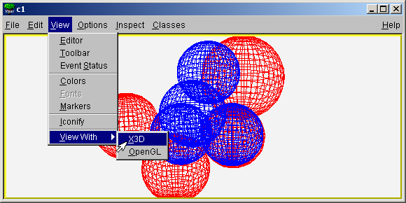
Invoking external 3D viewers from canvas menus
Note: A current limitation means that when an external viewer is created the pad is no longer redrawn. When the external viewer is closed, clicking in the pad will refresh.
The GL Viewer uses
The GL Viewer is supported on all official ROOT platforms (assuming you have suitable $ROOTSYS/gl.
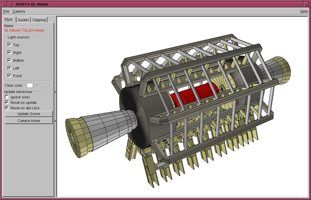
The GL 3D Viewer
You can manipulate the viewer via the GUI or via the base TGLViewer object behind the interface. These are detailed below - see also $ROOTSYS/tutorials/gl/glViewerExercise.C.
The GL Viewer supports two basic types of camera, which affect how the 3D world is projected onto the 2D render area:
Perspective: Objects are drawn with characteristic ‘foreshortening’ effect, where distant objects appear smaller than near ones. This is useful for obtaining a ‘real world’ views. The degree of foreshortening is affected by the current camera field of view (focal length of its ‘lens’) - see “Adjusting Cameras”.
Orthographic: Distance from camera does not affect object size. These projections are useful for measurement or checking alignments, as the sizes and angles between objects are preserved.
You can select the active camera from the viewer’s Camera menu on the top menu bar. There are three perspective camera choices:
Perspective (Floor XOZ) Default
Perspective (Floor YOZ)
Perspective (Floor XOY)
In each case the perspective camera is constrained to keep the chosen floor plane, defined by a pair of world axes, appearing level at all times - i.e. there is no banking of the ‘horizon’ that you experience when a plane rolls. There are also three orthographic camera choices:
Orthographic (XOY)
Orthographic (XOZ)
Orthographic (ZOY)
Orthographic projections are generally constrained to look down one of the global axes of the world, with the other two axes lying horizontal/vertical on the viewer window. Therefore, XOY has the X-axis horizontal, the Y-axis vertical. You can always confirm the orientation and constraints of the camera in the world by enabling axis drawing in the “Guides” tab - see sections “Guides” and “Clipping” below. For orthographic camera a ruler-depicting current scene units is also available.
You can also pick the current camera by obtaining a handle to the GL Viewer object behind the interface:
TGLViewer * v = (TGLViewer *)gPad->GetViewer3D();calling the method TGLViewer::SetCurrentCamera with one of the TGLViewer::ECameraType types:
v->SetCurrentCamera(TGLViewer::kCameraPerspXOZ);See also $ROOTSYS/tutorials/gl/glViewerExercise.C.
The interactions with the camera are summarized above. In each case the interaction is listed, along with description and user actions required to achieve it. For all cameras you can reset the original default view, framing the entire scene, by double clicking any mouse button.

GL Viewer camera interactions
For the Zoom interaction you can use the following modifiers combinations to adjust the sensitivity:
Shiftx 10
Ctrlx 0.1
Shift + Ctrlx 0.01
The modifiers must be applied after the zoom action has started (right mouse button is down).
Note for orthographic cameras:
There is no field of view of view/focal length - dollying and zooming producing an identical scaling action.
There is a fixed eye direction - so the ‘Orbit’ action is disabled.
Note for perspective cameras:
Dollying (moving the camera backwards/forwards) and zooming are often confused, and may appear very similar.
When you dolly the camera the lens focal length does not change, hence the distortions associated with the projections are unaffected. However the movement can result in objects coming ‘through the front’ of the camera and disappearing.
When you zoom, the camera does not move - hence clipping of near objects is unaffected. However with extremely small zooms (FOV large/focal length short) noticeable distortions, causing straight lines to become curved, can be seen with objects near the camera - the ‘fisheye’ lens effect.
Generally dollying is more ‘natural’, but you may need to use both to achieve the desired perspective and eye position - particularly when you are working inside or very close to 3D objects.
Configure the camera by calling the methods SetPerspectiveCamera() or SetOrthographicCamera() of TGLViewer:
TGLViewer * v = (TGLViewer *)gPad->GetViewer3D();
v->SetOrthoCamera(TGLViewer::kCameraOrthoXOY,
                  left,right,top,bottom);
...
v->SetPerspectiveCamera (camera,fov,dolly,center,hRotate,vRotate);
Note - you can configure any of the six cameras in the viewer at any time, but you will not see the result until the camera is made current.
The GL Viewer supports three different rendering modes, which are applied to all the objects in your scene, but not Clip Shapes and Guides (See “Clipping” and “Manipulators”). These are shown below, along with the key used to activate the style.
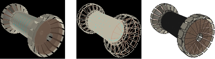
GL Viewer draw styles
Filled Polygons Wireframe Outline Enable with ‘r’ key Enable with ‘w’ key Enable with ‘t’ key Solid polygons, with hidden surface Object edges in color, with Combination of Filled Polygons removal, color surface materials, no surface filling/hiding. and Outline styles. Solid opacity, specular reflection etc. shapes with edges. Black background. Black background. White background.
Call method TGLViewer::SetStyle with one of TGLRnrCtx::EDrawStyleflags kFill, kOutline, kWireFrame:
v->SetStyle(TGLRnrCtx::kFill);The GL viewer creates five diffuse lights (left, right, top, bottom, and front) arranged around the 3D scene. These lights are carried with the camera - that is they are always in same position relative to your eye - the left light always shines from the left.
Light controls are located: Viewer Controls Pane ‘Style’.
Each light has a checkbox to enable/disable it. Set lights on/off with TGLLightSet::SetLight e.g.
v->GetLightSet()->SetLight(TGLLightSet::kLightBottom, kFALSE);The GL viewer supports interactive clipping, enabling you to remove sections of your 3D scene and the shapes, revealing internal details.
GL Viewer interactive box clipping
The controls for clipping can be found under: Viewer Controls Pane ‘Clipping’ tab.
Two clipping ‘shapes’ are currently supported:
Single plane
Box
Pick the type from the radio buttons - only one (or none) may be active at one time.
The clip object can be adjusted by:
Adjusting the values in the properties panel GUI
Directly manipulating the clip object in the viewer
To show and/or directly manipulate the object check the ‘Show / Edit in Viewer’ checkbox. The clip object is drawn in semi-transparent light brown. The current manipulator is attached to it, allowing you direct control over its position, scale and rotation. See “Manipulators” section below for details on using viewer manipulators.
The clip plane is described by the standard plane equation: ax+by+cz+d=0, where the factors a, b, c, d are entered into the edit boxes, and applied using the ‘Apply’ button.
The clip box is described by its center position, entered in the ‘Center X’, ‘Center Y’ and ‘Center Z’ edit boxes, and its lengths (extents) entered in the ‘Length X’, ‘Length Y’ and ‘Length Z’ edit boxes.
This clipping is achieved using OpenGL clip plane support; as such, there are certain limitations:
Solid shapes are not capped - they appear hollow.
Only shapes, which can be described with combination of planes, can be rendered in this fashion - e.g. a clipping tube is not possible.
Each additional clipping plane requires an additional render pass - so the more active planes the more time the render will take.
Set the current clip object with TGLClipSet::SetClipType
v->GetClipSet()->SetClipType(TGLClipSet::kClipPlane);Configure the clip object with TGLClipSet::SetClipState
Double_t planeEq[4] = {0.5,1.0,-1.0, 2.0};
v->GetClipSet()->SetClipState(TGLClipSet::kClipPlane, planeEq);
As with cameras, any clip can be configured at any time, but you must set the clip current to see the effect.
Manipulators are GUI ‘widgets’ or controls attached to a 3D object in the viewer, allowing a direct manipulation of the object’s geometry. There are three manipulators for the three basic geometries transformations. In each case, the manipulator consists of three components, one for each local axis of the object, shown in standard colors: red (X), green (Y) and blue (Z).
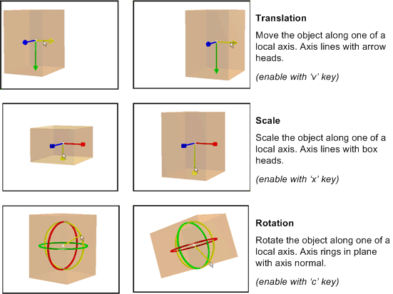
GL Viewer object manipulators
Activate the manipulator by moving the mouse over one of these components (which turns yellow to indicate active state). Click with left mouse and drag this active component to perform the manipulation. Toggle between the manipulator types using the ‘x’, ‘c’, ‘v’ keys while the mouse cursoris above the manipulator. Note: Manipulators cannot be controlled via the API at present.
Guides are visual aids drawn into the viewer world. Controls for these are under the “Guides” tab:
Viewer Controls Pane Guides Tab
Axes show the world (global) frame coordinatedirections: X (red), Y (green) and Z (blue). The negative portion of the axis line is shown in dark color, the positive in bright. The axis name and minimum / maximum values are labeled in the same color. There are three options for axes drawing - selected by radio buttons:
None - not drawn (default).
Edge - draw axes on the (minimum) edge of the scene extents box.
Origin - drawn axes through the origin.
For edge axes, the zero value for each axis is marked on the axis line with a colored sphere. For origin axes, a single white sphere is shown at the origin.
Edge axes are depth clipped - i.e. are obscured by 3D objects in front of them. Origin axes (which generally pass through the middle of the 3D scene) are not depth clipped - so always visible.
A single orange sphere of fixed view port (window) size can be shown at any arbitrary position. Enable / disable the drawing with ‘Show’ checkbox. Enter X/Y/Z position in the edit boxes to set position. Initial position is at the center of the scene.
Set the guides using TGLViewer::SetGuideState e.g. to enable edge axes, and enable a reference marker at world position 50, 60, 100:
Double_t refPos[3] = {50.0,60.0,100.0};
v->SetGuideState(TGLUtil::kAxesEdge, kTRUE, refPos);You can select a single shape from your scene by pressing ‘Shift’ key, pointing and left clicking anywhere on the shape in the viewer. Selection is currently shown by drawing the shape-bounding box (not depth clipped) in white (polygon or wire frame render styles) or red (outline render style). Manipulators supported by the shape are drawn in red, green and blue while the non-supported ones are drawn in grey. To deselect a shape, either select another, or shift/click anywhere on the background (empty space) in the viewer. You cannot select Manipulators or Guides (Axes / Reference Marker).
When a shape is selected, the viewer’s control pane shows the user interface that allows you to review and adjust the color and geometry properties of the shape.
Note: At present modifications to the shapes are local to the viewer - they are not propagated back to external objects/client that published to the viewer. The changes are preserved only until the viewer is closed. In some cases, this will never be feasible as there is not a one-to-one correspondence between a shape in the viewer and a single external object in which the modification could be stored.
Viewer Controls Pane ‘Style’ tab.
A full description of OpenGL materials, colors and lighting is beyond the scope of this document. You should refer to the OpenGL programming manual (Red Book) for a full discussion. In most cases adjustment of the Diffuse color material + Opacity/Shine properties is sufficient to achieve desired results.
A shape has four-color materials (components):
Diffuse
Ambient
Specular
Emissive
For each of these you can select the component via the radio buttons. Each component can have the red, green and blue values for the component adjusted via the sliders. You can apply this adjustment to the shape itself, or to all shapes sharing a common ‘family’. Shapes of the same family have external objects with the same TObject name string. You can also adjust the ‘Opacity’ and ‘Shine’ for the shapes materials via the sliders.
Viewer Controls Pane ‘Geometry’ tab.
Review and modify the shapes X/Y/Z center and scaling factors via the edit boxes. Selection and editing of shapes is not available via the API at present.
The current viewer rendering can be output to an external EPS or PDF, using the options under the ‘File’ menu on the top menu bar. The file is named ‘viewer.eps’ or ‘viewer.pdf’ and written to the current ROOT directory.
The X3D viewer is a fairly simple and limited viewer, capable of showing basic lines and polygons. It lacks the quality, performance and more advanced features of the GL Viewer, and additionally is not supported on Windows. It is not actively developed and you are encouraged to use the GL Viewer out of preference. The below table presents the main interactions - these are repeated in the Help dialog of the viewer.
Action KeyActionKey
Wireframe Mode wRotate about xx a
Hidden Line Mode eRotate about yy b
Hidden Surface Mode rRotate about zz c
Move object down uAuto-rotate about x1 2 3
Move object up iAuto-rotate about y4 5 6
Move object left lAuto-rotate about z7 8 9
Move object right hToggle controls styleo
Move object forward jToggle stereo displays
Move object backward kToggle blue stereo viewd
Adjust focus (stereo mode) [ ] { }Toggle double bufferf
Rotate object Left mouse button down + move.
The 3D Viewer Architecture provides a common mechanism for viewer clients to publish 3D objects to it. It enables:
Decoupling of producers (geometry packages etc) who model collection of 3D objects from consumers (viewers) which display them.
Producer code free of explicit drawing commands & viewer specific branching.
Support differing viewers and clients capabilities, e.g.
Mix of native (in viewer) shapes and generic client side tessellation.
Local/global frame object description
Bounding boxes
Placing copies sharing common geometry (logical/physical shapes).
The architecture consists of:
TVirtualViewer3D interface: An abstract handle to the viewer, allowing client to add objects, test preferences etc.
TBuffer3D class hierarchy: Used to describe 3D objects (“shapes”) - filled /added by negotiation with viewer via TVirtualViewer3D.
A typical interaction between viewer and client using these, taken from TGeoPainter is:
TVirtualViewer3D * viewer = gPad->GetViewer3D();
// Does viewer prefer local frame positions?
Bool_t localFrame = viewer->PreferLocalFrame();
// Perform first fetch of buffer from the shape and try adding it to the viewer
const TBuffer3D &buffer = shape.GetBuffer3D(TBuffer3D::kCore |
TBuffer3D::kBoundingBox |
TBuffer3D::kShapeSpecific,
localFrame);
Int_t reqSections = viewer->AddObject(buffer, &addDaughters);

// If the viewer requires additional sections fetch from the shape
// (if possible) and add again
if (reqSections != TBuffer3D::kNone)
shape.GetBuffer3D(reqSections, localFrame);
Together these allow clients to publish objects to any one of the 3D viewers free of viewer specific drawing code. They allow our simple x3d viewer, and considerably more sophisticated OpenGL one to both work with both geometry libraries (g3d and geom) efficiently.
In addition to external viewers, created in separate windows, this architecture is also used by internal TPad drawing when it requires 3D projections. Publishing to a viewer consists of the following steps:
1- Create / obtain viewer handle.
2- Begin scene on viewer.
3- Fill mandatory parts of TBuffer3D describing object.
4- Add to viewer.
5- Fill optional parts of TBuffer3D as requested by viewer.
[ …. repeat 3/4/5 as required for other/child objects]
6- End scene on viewer.
You should attach the top-level node of your external geometry (or the manager) to a TPad object using TObject::Draw(), and perform the publishing to the viewer in your object’s TObject::Paint() overloaded method. See “Scene Rebuilds”, and example scripts, for more details.
External viewers are bound to a TPad object (this may be removed as a requirement in the future). You can create or obtain the current viewer handle via the method:
TVirtualViewer3D * v = gPad->GetViewer3D("type");Here the “type” string defines the viewer type - currently one of:
“ogl” : External GL viewer
“x3d”: External X3D viewer
“pad”: Pad viewer
If no type is passed (null string), and there is no current viewer, then the type is defaulted to “pad”. If no type is passed and there is a current viewer, then this is returned - hence once a viewer is created it can be obtained elsewhere by:
TVirtualViewer3D * v = gPad->GetViewer3D();Objects must be added to viewer between BeginScene() and EndScene() calls e.g.
viewer->BeginScene();
// Add objects
viewer ->EndScene();
These calls enable the viewer to suspend redraws, and perform internal caching/setup. If the object you attach to the pad derives from TAtt3D, then the pad will take responsibility for calling BeginScene() and EndScene() for you. You can always test if the scene is already open for object addition with:
viewer->BuildingScene();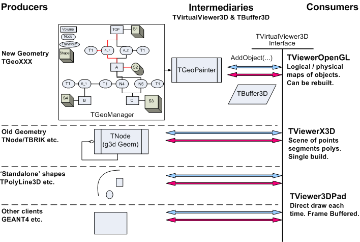
Overview of 3D viewer architecture
Note: the x3d viewer does not support rebuilding of scenes - objects added after the first Open/Close Scene pair will be ignored.
The viewers behind the TVirtualViewer3D interface differ greatly in their capabilities e.g.
Some support native shape (e.g. spheres/tubes in OpenGL) and can draw these based on an abstract description. Others always require a tessellation description based on TBuffer3D’s kRaw / kRawSizes points/lines/segments sections.
Some need the 3D object positions in the master (world) frame, others can cope with local frames and a translation matrix to place the object.
Some require bounding boxes for objects - others do not.
Similarly some viewer clients are only capable of providing positions in master frame, cannot provide bounding boxes etc. Additionally we do not want to incur the cost of expensive tessellation operations if the viewer does not require them. To cope with these variations the TBuffer3D objects are filled by negotiation with the viewer.
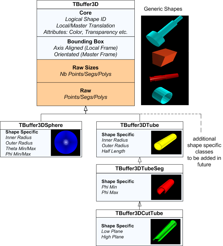
TBuffer3D class hierarchy
TBuffer3D classes are conceptually divided into enumerated sections: kCore, kBoundingBox, kRaw - see the class diagram and the file TBuffer3D.h for more details. The TBuffer3D methods SectionsValid(), SetSectionsValid(), ClearSectionsValid() are used to test, set, clear these section validity flags e.g.
buffer.SetSectionsValid(TBuffer3D::kShapeSpecific);
...
if (buffer.SectionsValid(TBuffer3D:: kShapeSpecific)) {
   ...
}
The sections found in the base TBuffer3D (kCore/kBoundingBox/kRawSizes/kRaw) are sufficient to describe any tessellated shape in a generic fashion. An additional kShapeSpecific section is added in TBuffer3D derived classes, allowing a more abstract shape description (“a sphere of inner radius x, outer radius y”). This enables a viewer, which knows how to draw (tessellate) the shape itself to do so, while providing a generic fallback suitable for all viewers. The rules for client negotiation with the viewer are:
If suitable specialized TBuffer3D class exists, use it, otherwise use TBuffer3D.
Complete the mandatory kCore section.
Complete the kShapeSpecific section if applicable.
Complete the kBoundingBox if you can.
Pass this buffer to the viewer using one of the TBuffer3D::AddObject() methods.
If the viewer requires more sections to be completed (kRaw/kRawSizes) TBuffer3D::AddObject() will return flags indicating which ones, otherwise it returns kNone. If requested, you must fill the buffer, mark these sections valid, and call TBuffer3D::AddObject again, to complete adding the object. For example, in out TGeo geometry package, in TGeoPainter::PaintShape, we perform the negotiation with viewer:
TVirtualViewer3D * viewer = gPad->GetViewer3D();
if (shape.IsA() != TGeoCompositeShape::Class()) {
   // Does viewer prefer local frame positions?
   Bool_t localFrame = viewer->PreferLocalFrame();
   // Perform first fetch of buffer from the shape and adding
   // it to the viewer
   const TBuffer3D &buffer = shape.GetBuffer3D(TBuffer3D::kCore |
   TBuffer3D::kBoundingBox |
   TBuffer3D::kShapeSpecific, localFrame);
   Int_t reqSections = viewer->AddObject(buffer, &addDaughters);
   // If the viewer requires additional sections fetch from the
   // shape (if possible) and add again
   if (reqSections != TBuffer3D::kNone) {
      shape.GetBuffer3D(reqSections, localFrame);
      viewer->AddObject(buffer, &addDaughters);
   }
}
The buffer is supplied/filled by the appropriate TShape::GetBuffer3D() and TShape::FillBuffer3D overloads e.g. for a sphere in TGeoSphere.
const TBuffer3D &TGeoSphere::GetBuffer3D(Int_t reqSections,
Bool_t localFrame) const {
   // Fills a static 3D buffer and returns a reference.
   static TBuffer3DSphere buffer;
   // Filling of kBoundingBox is defered to TGeoBBox, and
   // kCore on up to TGeoShape
   TGeoBBox::FillBuffer3D(buffer, reqSections, localFrame);
   // Complete kShapeSpecific section for sphere
   if (reqSections & TBuffer3D::kShapeSpecific) {
      buffer.fRadiusInner  = fRmin;
      buffer.fRadiusOuter  = fRmax;
      ...
      buffer.SetSectionsValid(TBuffer3D::kShapeSpecific);
   }
   // Complete kRawSizes section
   if (reqSections & TBuffer3D::kRawSizes) {
      ...
      buffer.SetSectionsValid(TBuffer3D::kRawSizes);
   }
}
   // Complete kRaw tesselation section
   if ((reqSections & TBuffer3D::kRaw) &&
        buffer.SectionsValid(TBuffer3D::kRawSizes)) {
      SetPoints(buffer.fPnts);
      // Transform points to master frame if viewer requires it
      // The fLocalFrame flag and translation matrix will have
      // already been set in TGeoShape::FillBuffer3D() as required
      if (!buffer.fLocalFrame)
         TransformPoints(buffer.fPnts, buffer.NbPnts());
      SetSegsAndPols(buffer);
      buffer.SetSectionsValid(TBuffer3D::kRaw);
   }
   return buffer;
}
Note:
we use a static TBuffer3D derived object for efficiency - once the object is added the buffer can be reused.
kRawSize (the calculation of tessellation sizing required in buffer) and kRaw (the actual filling of tessellation) is split, as the X3D viewer requires two publication passes - one to establish the full tessellation capacity for all shapes, and another to actually add them. Splitting avoids having to do the expensive tessellation on the first pass.
Currently we provide the following shape specific classes, which the GL Viewer can take advantage of (see TBuffer3D.h and TBuffer3DTypes.h)
TBuffer3DSphere - solid, hollow and cut spheres (GL Viewer only supports solid spheres at present - cut / hollow ones will be requested as tessellated objects by client.)
TBuffer3DTube - basic tube with inner/outer radius and length.
TBuffer3DTubeSeg - angle tube segment.
TBuffer3DCutTube - angle tube segment with plane cut ends.
See the above example from TGeoSphere::GetBuffer3D and also equivalent functions in TGeoTube, TGeoTubeSeg and TGeoCtub. Anyone is free to add new TBuffer3D classes, but it should be clear that one or more viewers will require updating to be able to take advantage of them. Hence we only provide classes which existing viewers can benefit from. The number of native shapes in GL Viewer will be expanded in the future.
The Core section of TBuffer3D contains two members relating to reference frames:
fLocalFrame: indicates if any positions in the buffer (bounding box and tessellation vertexes) are in local or master (world frame).
fLocalMaster: is a standard 4x4 translation matrix (OpenGL column major ordering) for placing the object into the 3D master frame.
If fLocalFrame is false, fLocalMaster should contain an identity matrix. This is set by default, and can be reset using the TBuffer3D::SetLocalMasterIdentity() method.
You are not obliged to complete the kBoundingBox section, as any viewer requiring one internally (GL Viewer) will build it if you do not provide. However to do this the viewer will force you to provide the (expensive) raw tessellation, and the resulting box will be axis aligned with the overall scene, which is non-ideal for rotated shapes. As we need to support orientated (rotated) bounding boxes, TBuffer3D requires the 6 vertices of the box. We also provide a convenience function, TBuffer::SetAABoundingBox(), for simpler case of setting an axis aligned bounding box. The bounding box should be filled in same frame (local / master) as the rest of the TBuffer3D, and inaccordance with fLocalFrame flag.
A typical example from TGeoBBox::FillBuffer3D:
   if (reqSections & TBuffer3D::kBoundingBox) {
      Double_t halfLengths[3] = { fDX, fDY, fDZ };
      buffer.SetAABoundingBox(fOrigin, halfLengths);
      if (!buffer.fLocalFrame) {
         TransformPoints(buffer.fBBVertex[0], 8);
      }
      buffer.SetSectionsValid(TBuffer3D::kBoundingBox);
}Some viewers can support two types of object placement:
Add object as a single independent entity in the world reference frame - e.g. a sphere, radius r, at x, y, z.
Repeated placement (copying) in world frame of this locally unique piece of geometry (described in local reference frame) e.g. define a sphere S (radius r), place copy at x1, y1, z1, another copy at x2, y2, z2 etc.
The second case is very typical in geometry packages, e.g. ROOT’s TGeo package, GEANT4 etc, where we have very large number repeated placements of relatively few unique “shapes”.
Some viewers (GL Viewer only at present) are able to take advantage of this by identifying unique logical shapes from the fID logical ID member of TBuffer3D. If repeated addition of the same fID is found, the shape is cached already - and the costly tessellation does not need to be sent again. The viewer can also perform internal GL specific caching (display lists) with considerable performance gains in these cases. For this to work correctly the logical object in must be described in TBuffer3D in the local reference frame, complete with the local/master translation. In some cases you will not have a real object you can reasonably set TBuffer3D::fID to, or the object is recycled or temporary. To suppress internal caching in the GL Viewer in these cases, set TBuffer3D::fID to 0 (null).
The viewer indicates it can support local frame objects through the TVirtualViewer3D interface method: PreferLocalFrame(). If this returns kTRUE you can make repeated calls to AddObject(), with TBuffer3D containing the same fID, and different fLocalMaster placements.
For viewers supporting logical/physical objects, the TBuffer3D content refers to the properties of the logical object, with the exception of:
fLocalMaster transform
fColor
fTransparency
attributes, which can be varied for each physical object.
As a minimum requirement all clients must be capable of filling the raw tessellation of the object buffer, in the master reference frame. Conversely viewers must always be capable of displaying the object described by this buffer. If either does not meet this requirement the object may not be displayed.
TBuffer3D::AddObject is not an explicit command to the viewer - it may for various reasons decide to ignore it:
It already has the object internally cached.
The object falls outside some ‘interest’ limits of the viewer camera.
The object is too small to be worth drawing.
In all these cases TBuffer3D::AddObject() returns kNone, as it does for successful addition, indicating it does not require further information about this object. Hence you should not try to make any assumptions about what the viewer did with the object. The viewer may decide to force the client to rebuild (republish) the scene, obtaining a different collection of objects, if the internal viewer state changes .e.g. significant camera move. It does this presently by forcing a repaint on the attached TPad object - hence you should attach you master geometry object to the pad (via TObject::Draw()), and perform the publishing to the viewer in response to TObject::Paint().
TVirtualViewer3D provides for two methods of object addition:
virtual Int_t AddObject(const TBuffer3D &buffer,
                        Bool_t * addChildren = 0)
virtual Int_t AddObject(UInt_t physicalID,
                        const TBuffer3D & buffer,
                        Bool_t *addChildren = 0)
If you use the first (simple) case a viewer using logical/physical pairs will generate sequential IDs for each physical object internally. Scene rebuilds will require destruction and recreation of all physical objects. For the second you can specify an identifier from the client side, which must be unique and stable - i.e. the IDs of a published object is consistent, regardless of changes in termination of contained child geometry branches. In this case the viewer can safely cache the physical objects across scene rebuilds, discarding those no longer of interest.
In many geometries there is a rigid containment hierarchy, and so if the viewer is not interested in a certain object due to limits/size then it will also not be interest in any of the contained branch of siblings. Both TBuffer3D::AddObject() methods have an addChildren return parameter. The viewer will complete this (if passed) indicating if children of the object just sent are worth sending.
Once add TBuffer3D::AddObject() has been called, the contents are copied to the viewer’s internal data structures. You are free to destroy this TBuffer3D, or recycle it for the next object if suitable.
For an example of a simple geometry, working in master reference frame examine the code under $ROOTSYS/g3d. For a more complex example, which works in both master and local frames, and uses logical/physical division of shape geometry and placement, examine the code under $ROOTSYS/geom - in particular TGeoShape hierarchy, and the painter object TGeoPainter (under geopainter) where the negotiation with the viewer is performed.