WARNING: This documentation is not maintained anymore. Some part might be obsolete or wrong, some part might be missing but still some valuable information can be found there. Instead please refer to the ROOT Reference Guide and the ROOT Manual. If you think some information should be imported in the ROOT Reference Guide or in the ROOT Manual, please post your request to the ROOT Forum or via a Github Issue.
% Chapter: Histograms ________________________________________________________________________________________ WARNING: This documentation is not maintained anymore. Some part might be obsolete or wrong, some part might be missing but still some valuable information can be found there. Instead please refer to the ROOT Reference Guide and the ROOT Manual. If you think some information should be imported in the ROOT Reference Guide or in the ROOT Manual, please post your request to the ROOT Forum or via a Github Issue.
% Chapter: Histograms ________________________________________________________________________________________ WARNING: This documentation is not maintained anymore. Some part might be obsolete or wrong, some part might be missing but still some valuable information can be found there. Instead please refer to the ROOT Reference Guide and the ROOT Manual. If you think some information should be imported in the ROOT Reference Guide or in the ROOT Manual, please post your request to the ROOT Forum or via a Github Issue.
This chapter covers the functionality of the histogram classes. We begin with an overview of the histogram classes, after which we provide instructions and examples on the histogram features.
We have put this chapter ahead of the graphics chapter so that you can begin working with histograms as soon as possible. Some of the examples have graphics commands that may look unfamiliar to you. These are covered in the chapter “Input/Output”.
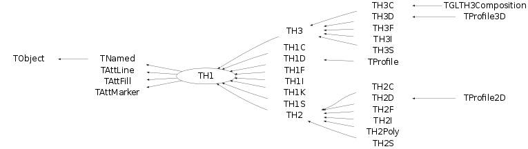
ROOT supports histograms up to three dimensions. Separate concrete classes are provided for one-dimensional, two-dimensional and three-dimensional classes. The histogram classes are split into further categories, depending on the set of possible bin values:
TH1C, TH2C and TH3C contain one char (one byte) per bin (maximum bin content = 255)
TH1S, TH2S and TH3S contain one short (two bytes) per bin (maximum bin content = 65 535).
TH1I, TH2I and TH3I contain one integer (four bytes) per bin (maximum bin content = 2 147 483 647).
TH1L, TH2L and TH3L contain one long64 (eight bytes) per bin (maximum bin content = 9 223 372 036 854 775 807).
TH1F, TH2F and TH3F contain one float (four bytes) per bin (maximum precision = 7 digits).
TH1D, TH2D and TH3D contain one double (eight bytes) per bin (maximum precision = 14 digits).
ROOT also supports profile histograms, which constitute an elegant replacement of two-dimensional histograms in many cases. The inter-relation of two measured quantities X and Y can always be visualized with a two-dimensional histogram or scatter-plot. Profile histograms, on the other hand, are used to display the mean value of Y and its RMS for each bin in X. If Y is an unknown but single-valued approximate function of X, it will have greater precision in a profile histogram than in a scatter plot.
TProfile : one dimensional profiles
TProfile2D : two dimensional profiles
All ROOT histogram classes are derived from the base class TH1 (see figure above). This means that two-dimensional and three-dimensional histograms are seen as a type of a one-dimensional histogram, in the same way in which multidimensional C arrays are just an abstraction of a one-dimensional contiguous block of memory.
There are several ways in which you can create a histogram object in ROOT. The straightforward method is to use one of the several constructors provided for each concrete class in the histogram hierarchy. For more details on the constructor parameters, see the subsection “Constant or Variable Bin Width” below. Histograms may also be created by:
Calling the Clone() method of an existing histogram
Making a projection from a 2-D or 3-D histogram
Reading a histogram from a file (see Input/Output chapter)
   // using various constructors
   TH1* h1 = new TH1I("h1", "h1 title", 100, 0.0, 4.0);
   TH2* h2 = new TH2F("h2", "h2 title", 40, 0.0, 2.0, 30, -1.5, 3.5);
   TH3* h3 = new TH3D("h3", "h3 title", 80, 0.0, 1.0, 100, -2.0, 2.0,
                       50, 0.0, 3.0);

   // cloning a histogram
   TH1* hc = (TH1*)h1->Clone();

   // projecting histograms
   // the projections always contain double values !
   TH1* hx = h2->ProjectionX(); // ! TH1D, not TH1F
TH1* hy = h2->ProjectionY(); // ! TH1D, not TH1FThe histogram classes provide a variety of ways to construct a histogram, but the most common way is to provide the name and title of histogram and for each dimension: the number of bins, the minimum x (lower edge of the first bin) and the maximum x (upper edge of the last bin).
   TH2* h = new TH2D(
      /* name */ "h2",
      /* title */ "Hist with constant bin width",
      /* X-dimension */ 100, 0.0, 4.0,
      /* Y-dimension */ 200, -3.0, 1.5);
When employing this constructor, you will create a histogram with constant (fixed) bin width on each axis. For the example above, the interval [0.0, 4.0] is divided into 100 bins of the same width w X = 4.0 - 0.0 100 = 0.04 for the X axis (dimension). Likewise, for the Y axis (dimension), we have bins of equal width w Y = 1.5 - (-3.0) 200 = 0.0225.
If you want to create histograms with variable bin widths, ROOT provides another constructor suited for this purpose. Instead of passing the data interval and the number of bins, you have to pass an array (single or double precision) of bin edges. When the histogram has n bins, then there are n+1 distinct edges, so the array you pass must be of size n+1.
   const Int_t NBINS = 5;
   Double_t edges[NBINS + 1] = {0.0, 0.2, 0.3, 0.6, 0.8, 1.0};
   // Bin 1 corresponds to range [0.0, 0.2]
   // Bin 2 corresponds to range [0.2, 0.3] etc...

   TH1* h = new TH1D(
      /* name */ "h1",
      /* title */ "Hist with variable bin width",
      /* number of bins */ NBINS,
      /* edge array */ edges
    );
Each histogram object contains three TAxis objects: fXaxis , fYaxis, and fZaxis, but for one-dimensional histograms only the X-axis is relevant, while for two-dimensional histograms the X-axis and Y-axis are relevant. See the class TAxis for a description of all the access methods. The bin edges are always stored internally in double precision.
You can examine the actual edges / limits of the histogram bins by accessing the axis parameters, like in the example below:
   const Int_t XBINS = 5; const Int_t YBINS = 5;
   Double_t xEdges[XBINS + 1] = {0.0, 0.2, 0.3, 0.6, 0.8, 1.0};
   Double_t yEdges[YBINS + 1] = {-1.0, -0.4, -0.2, 0.5, 0.7, 1.0};

   TH2* h = new TH2D("h2", "h2", XBINS, xEdges, YBINS, yEdges);
   TAxis* xAxis = h->GetXaxis(); TAxis* yAxis = h->GetYaxis();

   cout << "Third bin on Y-dimension: " << endl; // corresponds to
                                                 // [-0.2, 0.5]
   cout << "\tLower edge: " << yAxis->GetBinLowEdge(3) << endl;
   cout << "\tCenter: " << yAxis->GetBinCenter(3) << endl;
cout << "\tUpper edge: " << yAxis->GetBinUpEdge(3) << endl;All histogram types support fixed or variable bin sizes. 2-D histograms may have fixed size bins along X and variable size bins along Y or vice-versa. The functions to fill, manipulate, draw, or access histograms are identical in both cases.
For all histogram types: nbins , xlow , xup
Bin# 0 contains the underflow.
Bin# 1 contains the first bin with low-edge ( xlow INCLUDED).
The second to last bin (bin# nbins) contains the upper-edge (xup EXCLUDED).
The Last bin (bin# nbins+1) contains the overflow.
In case of 2-D or 3-D histograms, a “global bin” number is defined. For example, assuming a 3-D histogram h with binx, biny, binz, the function returns a global/linear bin number.
This global bin is useful to access the bin information independently of the dimension.
At any time, a histogram can be re-binned via the TH1::Rebin() method. It returns a new histogram with the re-binned contents. If bin errors were stored, they are recomputed during the re-binning.
A histogram is typically filled with statements like:
   h1->Fill(x);
   h1->Fill(x,w); // with weight
   h2->Fill(x,y);
   h2->Fill(x,y,w);
   h3->Fill(x,y,z);
   h3->Fill(x,y,z,w);
The Fill method computes the bin number corresponding to the given x, y or z argument and increments this bin by the given weight. The Fill() method returns the bin number for 1-D histograms or global bin number for 2-D and 3-D histograms. If TH1::Sumw2() has been called before filling, the sum of squares is also stored. One can increment a bin number directly by calling TH1::AddBinContent(), replace the existing content via TH1::SetBinContent() , and access the bin content of a given bin via TH1::GetBinContent() .
By default, the number of bins is computed using the range of the axis. You can change this to re-bin automatically by setting the automatic re-binning option:
Once this is set, the Fill() method will automatically extend the axis range to accommodate the new value specified in the Fill() argument. The used method is to double the bin size until the new value fits in the range, merging bins two by two. The TTree::Draw() method extensively uses this automatic binning option when drawing histograms of variables in TTree with an unknown range. The automatic binning option is supported for 1-D, 2-D and 3-D histograms. During filling, some statistics parameters are incremented to compute the mean value and root mean square with the maximum precision. In case of histograms of type TH1C, TH1S, TH2C, TH2S, TH3C, TH3S a check is made that the bin contents do not exceed the maximum positive capacity (127 or 65 535). Histograms of all types may have positive or/and negative bin contents.
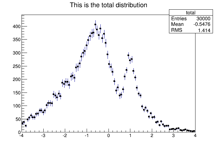
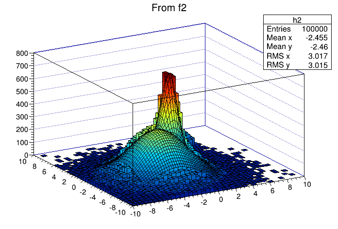
TH1::FillRandom() can be used to randomly fill a histogram using the contents of an existing TF1 function or another TH1 histogram (for all dimensions). For example, the following two statements create and fill a histogram 10 000 times with a default Gaussian distribution of mean 0 and sigma 1 :
TH1::GetRandom() can be used to get a random number distributed according the contents of a histogram. To fill a histogram following the distribution in an existing histogram you can use the second signature of TH1::FillRandom(). Next code snipped assumes that h is an existing histogram (TH1 ).
The distribution contained in the histogram h1 ( TH1 ) is integrated over the channel contents. It is normalized to one. The second parameter (1000) indicates how many random numbers are generated.
Getting 1 random number implies:
Generating a random number between 0 and 1 (say r1 )
Find the bin in the normalized integral for r1
Fill histogram channel
You can see below an example of the TH1::GetRandom() method which can be used to get a random number distributed according the contents of a histogram.
void getrandomh() {
   TH1F *source = new TH1F("source","source hist",100,-3,3);
   source->FillRandom("gaus",1000);
   TH1F *final = new TH1F("final","final hist",100,-3,3);

             // continued...

   for (Int_t i=0;i<10000;i++) {
      final->Fill(source->GetRandom());
   }
   TCanvas *c1 = new TCanvas("c1","c1",800,1000);
   c1->Divide(1,2);
   c1->cd(1);
   source->Draw();
   c1->cd(2);
   final->Draw();
   c1->cd();
}Many types of operations are supported on histograms or between histograms:
Addition of a histogram to the current histogram
Additions of two histograms with coefficients and storage into the current histogram
Multiplications and divisions are supported in the same way as additions.
The Add , Divide and Multiply methods also exist to add, divide or multiply a histogram by a function.
Histograms objects (not pointers) TH1F h1 can be multiplied by a constant using:
A new histogram can be created without changing the original one by doing:
To multiply two histogram objects and put the result in a 3rd one do:
The same operations can be done with histogram pointers TH1F *h1, *h2 following way:
Of course, the TH1 methods Add , Multiply and Divide can be used instead of these operators.
If a histogram has associated error bars ( TH1::Sumw2() has been called), the resulting error bars are also computed assuming independent histograms. In case of divisions, binomial errors are also supported.
One can make:
a 1-D projection of a 2-D histogram or profile. See TH2::ProfileX, TH2::ProfileY,TProfile::ProjectionX, TProfile2D::ProjectionXY, TH2::ProjectionX, TH2::ProjectionY .
a 1-D, 2-D or profile out of a 3-D histogram see TH3::ProjectionZ, TH3::Project3D.
These projections can be fit via: TH2::FitSlicesX, TH2::FitSlicesY, TH3::FitSlicesZ.
When you call the Draw method of a histogram ( TH1::Draw ) for the first time, it creates a THistPainter object and saves a pointer to painter as a data member of the histogram. The THistPainter class specializes in the drawing of histograms. It allows logarithmic axes (x, y, z) when the CONT drawing option is using. The THistPainter class is separated from the histogram so that one can have histograms without the graphics overhead, for example in a batch program. The choice to give each histogram has its own painter rather than a central singleton painter, allows two histograms to be drawn in two threads without overwriting the painter’s values. When a displayed histogram is filled again, you do not have to call the Draw method again. The image is refreshed the next time the pad is updated. A pad is updated after one of these three actions:
A carriage control on the ROOT command line
A click inside the pad
A call to TPad::Update()
By default, the TH1::Draw clears the pad before drawing the new image of the histogram. You can use the "SAME" option to leave the previous display intact and superimpose the new histogram. The same histogram can be drawn with different graphics options in different pads. When a displayed histogram is deleted, its image is automatically removed from the pad. To create a copy of the histogram when drawing it, you can use TH1::DrawClone(). This will clone the histogram and allow you to change and delete the original one without affecting the clone. You can use TH1::DrawNormalized() to draw a normalized copy of a histogram.
A clone of this histogram is normalized to norm and drawn with option. A pointer to the normalized histogram is returned. The contents of the histogram copy are scaled such that the new sum of weights (excluding under and overflow) is equal to norm .
Note that the returned normalized histogram is not added to the list of histograms in the current directory in memory. It is the user’s responsibility to delete this histogram. The kCanDelete bit is set for the returned object. If a pad containing this copy is cleared, the histogram will be automatically deleted. See “Draw Options” for the list of options.
Histograms use the current style gStyle, which is the global object of class TStyle. To change the current style for histograms, the TStyle class provides a multitude of methods ranging from setting the fill color to the axis tick marks. Here are a few examples:
   void SetHistFillColor(Color_t color = 1)
   void SetHistFillStyle(Style_t styl = 0)
   void SetHistLineColor(Color_t color = 1)
   void SetHistLineStyle(Style_t styl = 0)
   void SetHistLineWidth(Width_t width = 1)
When you change the current style and would like to propagate the change to a previously created histogram you can call TH1::UseCurrentStyle(). You will need to call UseCurrentStyle() on each histogram. When reading many histograms from a file and you wish to update them to the current style, you can use gROOT::ForceStyle and all histograms read after this call will be updated to use the current style. See “Graphics and the Graphical User Interface”. When a histogram is automatically created as a result of a TTree::Draw , the style of the histogram is inherited from the tree attributes and the current style is ignored. The tree attributes are the ones set in the current TStyle at the time the tree was created. You can change the existing tree to use the current style, by calling TTree::UseCurrentStyle() .
The following draw options are supported on all histogram classes:
“AXIS”: Draw only the axis.
“HIST”: When a histogram has errors, it is visualized by default with error bars. To visualize it without errors use HIST together with the required option (e.g. “HIST SAME C”).
“SAME”: Superimpose on previous picture in the same pad.
“CYL”: Use cylindrical coordinates.
“POL”: Use polar coordinates.
“SPH”: Use spherical coordinates.
“PSR”: Use pseudo-rapidity/phi coordinates.
“LEGO”: Draw a lego plot with hidden line removal.
“LEGO1”: Draw a lego plot with hidden surface removal.
“LEGO2”: Draw a lego plot using colors to show the cell contents.
“SURF”: Draw a surface plot with hidden line removal.
“SURF1”: Draw a surface plot with hidden surface removal.
“SURF2”: Draw a surface plot using colors to show the cell contents.
“SURF3”: Same as SURF with a contour view on the top.
“SURF4”: Draw a surface plot using Gouraud shading.
“SURF5”: Same as SURF3 but only the colored contour is drawn. Used with option CYL , SPH or PSR it allows to draw colored contours on a sphere, a cylinder or in a pseudo rapidly space. In Cartesian or polar coordinates, option SURF3 is used.
The following options are supported for 1-D histogram classes:
“AH”: Draw the histogram, but not the axis labels and tick marks
“B”: Draw a bar chart
“C”: Draw a smooth curve through the histogram bins
“E”: Draw the error bars
“E0”: Draw the error bars including bins with 0 contents
“E1”: Draw the error bars with perpendicular lines at the edges
“E2”: Draw the error bars with rectangles
“E3”: Draw a fill area through the end points of the vertical error bars
“E4”: Draw a smoothed filled area through the end points of the error bars
“L”: Draw a line through the bin contents
“P”: Draw a (poly)marker at each bin using the histogram’s current marker style
“P0”: Draw current marker at each bin including empty bins
“PIE”: Draw a Pie Chart
“*H”: Draw histogram with a * at each bin
“LF2”: Draw histogram as with option “L” but with a fill area. Note that “L” also draws a fill area if the histogram fill color is set but the fill area corresponds to the histogram contour.
“9”: Force histogram to be drawn in high resolution mode. By default, the histogram is drawn in low resolution in case the number of bins is greater than the number of pixels in the current pad
“][”: Draw histogram without the vertical lines for the first and the last bin. Use it when superposing many histograms on the same picture.
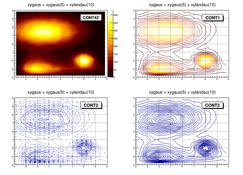
The following options are supported for 2-D histogram classes:
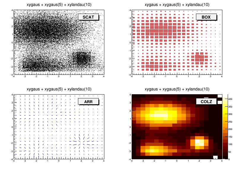
“ARR”: Arrow mode. Shows gradient between adjacent cells
“BOX”: Draw a box for each cell with surface proportional to contents
“BOX1”: A sunken button is drawn for negative values, a raised one for positive values
“COL”: Draw a box for each cell with a color scale varying with contents
“COLZ”: Same as “COL” with a drawn color palette
“CONT”: Draw a contour plot (same as CONT0 )
“CONTZ”: Same as “CONT” with a drawn color palette
“CONT0”: Draw a contour plot using surface colors to distinguish contours
“CONT1”: Draw a contour plot using line styles to distinguish contours
“CONT2”: Draw a contour plot using the same line style for all contours
“CONT3”: Draw a contour plot using fill area colors
“CONT4”: Draw a contour plot using surface colors (SURF2 option at theta = 0)
"CONT5": Use Delaunay triangles to compute the contours
“LIST”: Generate a list of TGraph objects for each contour
“FB”: To be used with LEGO or SURFACE , suppress the Front-Box
“BB”: To be used with LEGO or SURFACE , suppress the Back-Box
“A”: To be used with LEGO or SURFACE , suppress the axis
“SCAT”: Draw a scatter-plot (default)
“SPEC”: Use TSpectrum2Painter tool for drawing
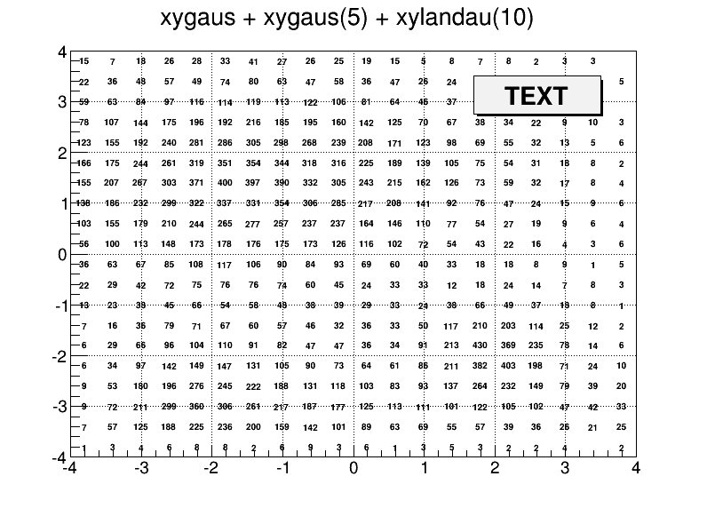
“TEXT”: Draw bin contents as text (format set via gStyle->SetPaintTextFormat) .
“TEXTnn”: Draw bin contents as text at angle nn ( 0<nn<90 ).
“[cutg]”: Draw only the sub-range selected by the TCutG name “cutg”.
“Z”: The “Z” option can be specified with the options: BOX, COL, CONT, SURF, and LEGO to display the color palette with an axis indicating the value of the corresponding color on the right side of the picture.
The following options are supported for 3-D histogram classes:
" " : Draw a 3D scatter plot.
“BOX”: Draw a box for each cell with volume proportional to contents
“LEGO”: Same as “BOX”
“ISO”: Draw an iso surface
“FB”: Suppress the Front-Box
“BB”: Suppress the Back-Box
“A”: Suppress the axis
Most options can be concatenated without spaces or commas, for example, if h is a histogram pointer:
The options are not case sensitive. The options BOX , COL and COLZ use the color palette defined in the current style (see TStyle::SetPalette). The options CONT , SURF , and LEGO have by default 20 equidistant contour levels, you can change the number of levels with TH1::SetContour. You can also set the default drawing option with TH1::SetOption . To see the current option use TH1::GetOption . For example:
   h->SetOption("lego");
   h->Draw(); // will use the lego option
h->Draw("scat") // will use the scatter plot optionBy default, 2D histograms are drawn as scatter plots. For each cell (i,j) a number of points proportional to the cell content are drawn. A maximum of 500 points per cell are drawn. If the maximum is above 500 contents are normalized to 500.
The ARR option shows the gradient between adjacent cells. For each cell (i,j) an arrow is drawn. The orientation of the arrow follows the cell gradient.
For each cell (i,j) a box is drawn with surface proportional to contents. The size of the box is proportional to the absolute value of the cell contents. The cells with negative contents are drawn with an X on top of the boxes. With option BOX1 a button is drawn for each cell with surface proportional to contents’ absolute value. A sunken button is drawn for negative values, a raised one for positive values.
"E" Default. Draw only error bars, without markers
"E0" Draw also bins with 0 contents (turn off the symbols clipping).
"E1" Draw small lines at the end of error bars
"E2" Draw error rectangles
"E3" Draw a fill area through the end points of vertical error bars
"E4" Draw a smoothed filled area through the end points of error bars
Note that for all options, the line and fill attributes of the histogram are used for the errors or errors contours. Use gStyle->SetErrorX(dx) to control the size of the error along x. The parameter dx is a percentage of bin width for errors along X. Set dx=0 to suppress the error along X. Use gStyle->SetEndErrorSize(np) to control the size of the lines at the end of the error bars (when option 1 is used). By default np=1 (np represents the number of pixels).
For each cell (i,j) a box is drawn with a color proportional to the cell content. The color table used is defined in the current style (gStyle ). The color palette in TStyle can be modified with TStyle::SetPalette .
For each cell (i,j) the cell content is printed. The text attributes are:
Text font = current font set by TStyle
Text size= 0.02 * pad-height * marker-size
Text color= marker color
The following contour options are supported:
"CONT": Draw a contour plot (same as CONT0)
"CONT0": Draw a contour plot using surface colors to distinguish contours
"CONT1": Draw a contour plot using line styles to distinguish contours
"CONT2": Draw a contour plot using the same line style for all contours
"CONT3": Draw a contour plot using fill area colors
"CONT4":Draw a contour plot using surface colors (SURF2 option at theta = 0); see also options “AITOFF”, “MERCATOR”, etc. below
"CONT5": Use Delaunay triangles to compute the contours
The default number of contour levels is 20 equidistant levels. It can be changed with TH1::SetContour. When option “LIST” is specified together with option “CONT”, all points used for contour drawing, are saved in the TGraph object and are accessible in the following way:
   TObjArray *contours =
      gROOT->GetListOfSpecials()->FindObject("contours");
   Int_t ncontours = contours->GetSize(); TList *list =
   (TList*)contours->At(i);
Where “i” is a contour number and list contains a list of TGraph objects. For one given contour, more than one disjoint poly-line may be generated. The TGraph numbers per contour are given by list->GetSize(). Here we show how to access the first graph in the list.
“AITOFF”: Draw a contour via an AITOFF projection
“MERCATOR”: Draw a contour via a Mercator projection
“SINUSOIDAL”: Draw a contour via a Sinusoidal projection
“PARABOLIC”: Draw a contour via a Parabolic projection
The tutorial macro earth.C uses these four options and produces the following picture:
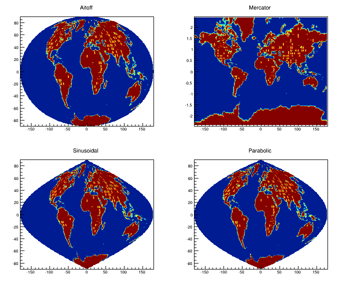
earth.C macro outputIn a lego plot, the cell contents are drawn as 3D boxes, with the height of the box proportional to the cell content.
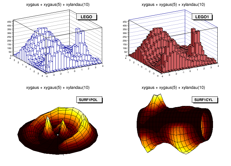
“LEGO”: Draw a lego plot with hidden line removal
“LEGO1”: Draw a lego plot with hidden surface removal
“LEGO2”: Draw a lego plot using colors to show the cell contents
A lego plot can be represented in several coordinate systems; the default system is Cartesian coordinates. Other possible coordinate systems are CYL , POL , SPH , and PSR .
“CYL”: Cylindrical coordinates: x-coordinate is mapped on the angle; y-coordinate - on the cylinder length.
“POL”: Polar coordinates: x-coordinate is mapped on the angle; y-coordinate - on the radius.
“SPH”: Spherical coordinates: x-coordinate is mapped on the latitude; y-coordinate - on the longitude.
“PSR”: PseudoRapidity/Phi coordinates: x-coordinate is mapped on Phi.
With TStyle::SetPalette the color palette can be changed. We suggest you use palette 1 with the call:
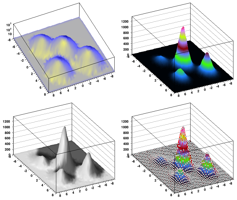
In a surface plot, cell contents are represented as a mesh. The height of the mesh is proportional to the cell content. A surface plot can be represented in several coordinate systems. The default is Cartesian coordinates, and the other possible systems are CYL, POL, SPH, and PSR . The following picture uses SURF1 . With TStyle::SetPalette the color palette can be changed. We suggest you use palette 1 with the call:
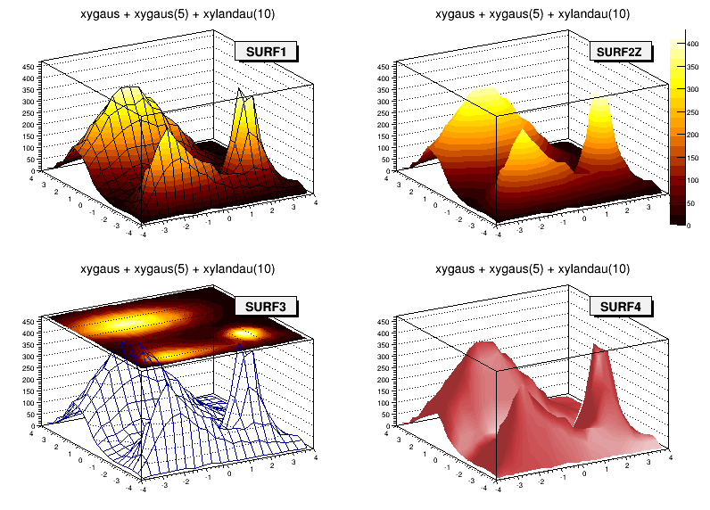
“SURF”: Draw a surface plot with hidden line removal
“SURF1”: Draw a surface plot with hidden surface removal
“SURF2”: Draw a surface plot using colors to show the cell contents
“SURF3”: Same as SURF with a contour view on the top
“SURF4”: Draw a surface plot using Gouraud shading
“SURF5”: Same as SURF3 but only the colored contour is drawn. Used with options CYL , SPH or PSR it allows to draw colored contours on a sphere, a cylinder or in a pseudo rapidly space. In Cartesian or polar coordinates, option SURF3 is used.
When the option “bar” or “hbar” is specified, a bar chart is drawn.
The options for vertical bar chart are “bar”, “bar0”, “bar1”, “bar2”, “bar3”, “bar4”.
"bar" or "bar0""bar1""bar2""bar3""bar4"Use TH1::SetBarWidth() to control the bar width (default is the bin width). Use TH1::SetBarOffset to control the bar offset (default is 0). See the example $ROOTSYS/tutorials/hist/hbars.C
The options for the horizontal bar chart are “hbar”, “hbar0”, “hbar1”, “hbar2”, “hbar3”, and “hbar4”.
hbar” or “hbar0”hbar1”hbar2”hbar3”hbar4”Use TH1::SetBarWidth to control the bar width (default is the bin width). Use TH1::SetBarOffset to control the bar offset (default is 0). See the example $ROOTSYS/tutorials/hist/hbars.C
The “Z” option can be specified with the options: COL, CONT, SURF, and LEGO to display the color palette with an axis indicating the value of the corresponding color on the right side of the picture. If there is not enough space on the right side, you can increase the size of the right margin by calling TPad::SetRightMargin(). The attributes used to display the palette axis values are taken from the Z axis of the object. For example, you can set the labels size on the palette axis with:
You can set the color palette with TStyle::SetPalette , e.g.
For example, the option COL draws a 2-D histogram with cells represented by a box filled with a color index, which is a function of the cell content. If the cell content is N, the color index used will be the color number in colors[N] . If the maximum cell content is greater than ncolors , all cell contents are scaled to ncolors. If ncolors<=0, a default palette of 50 colors is defined. This palette is recommended for pads, labels. It defines:
The color numbers specified in this palette can be viewed by selecting the menu entry Colors in the View menu of the canvas menu bar. The color’s red, green, and blue values can be changed via TColor::SetRGB.
If ncolors == 1 && colors == 0, then a Pretty Palette with a spectrum violet to red is created with 50 colors. That’s the default rain bow palette.
Other predefined palettes with 255 colors are available when colors == 0. The following value of ncolors (with colors = 0) give access to:
ncolors = 51 : Deep Sea palette.ncolors = 52 : Grey Scale palette.ncolors = 53 : Dark Body Radiator palette.ncolors = 54 : Two-color hue palette palette. (dark blue through neutral gray to bright yellow)ncolors = 55 : Rain Bow palette.ncolors = 56 : Inverted Dark Body Radiator palette.The color numbers specified in the palette can be viewed by selecting the item “colors” in the “VIEW” menu of the canvas toolbar. The color parameters can be changed via TColor::SetRGB.
Note that when drawing a 2D histogram h2 with the option “COL” or “COLZ” or with any “CONT” options using the color map, the number of colors used is defined by the number of contours n specified with: h2->SetContour(n)
A TPaletteAxisobject is used to display the color palette when drawing 2D histograms. The object is automatically created when drawing a 2D histogram when the option “z” is specified. It is added to the histogram list of functions. It can be retrieved and its attributes can be changed with:
The palette can be interactively moved and resized. The context menu can be used to set the axis attributes. It is possible to select a range on the axis, to set the min/max in z.
The “SPEC” option offers a large set of options/attributes to visualize 2D histograms thanks to “operators” following the “SPEC” keyword. For example, to draw the 2-D histogram h2 using all default attributes except the viewing angles, one can do:
The operators’ names are case insensitive (i.e. one can use “a” or “A”) and their parameters are separated by coma “,”. Operators can be put in any order in the option and must be separated by a space " ". No space characters should be put in an operator. All the available operators are described below.
The way how a 2D histogram will be painted is controlled by two parameters: the “Display modes groups” and the “Display Modes”. “Display modes groups” can take the following values:
“Display modes” can take the following values:
These parameters can be set by using the “dm” operator in the option.
The above example draws the histogram using the “Light Display mode group” and the “Grid Display mode”. The following tables summarize all the possible combinations of both groups:
| Points | Grid | Contours | Bars | LinesX | LinesY | |
| Simple | x | x | x | x | x | x |
| Light | x | x | x | x | ||
| Height | x | x | x | x | x | x |
| LightHeight | x | x | x | x |
| BarsX | BarsY | Needles | Surface | Triangles | |
| Simple | x | x | x | x | |
| Light | x | x | |||
| Height | x | x | x | x | |
| LightHeight | x | x |
The “Pen Attributes” can be changed using pa(color,style,width). Next example sets line color to 2, line type to 1 and line width to 2. Note that if pa() is not specified, the histogram line attributes are used:
The number of “Nodes” can be changed with n(nodesx,nodesy). Example:
Sometimes the displayed region is rather large. When displaying all channels the pictures become very dense and complicated. It is very difficult to understand the overall shape of data. “n(nx,ny)” allows to change the density of displayed channels. Only the channels coinciding with given nodes are displayed.
The visualization “Angles” can be changed with “a(alpha,beta,view)”: “alpha” is the angle between the bottom horizontal screen line and the displayed space on the right side of the picture and “beta” on the left side, respectively. One can rotate the 3-d space around the vertical axis using the “view” parameter. Allowed values are 0, 90, 180 and 270 degrees.
The operator “zs(scale)” changes the scale of the Z-axis. The possible values are:
If gPad->SetLogz() has been set, the log scale on Z-axis is set automatically, i.e. there is no need for using the zs() operator. Note that the X and Y axis are always linear.
The operator “ci(r,g,b)” defines the colors increments (r, g and b are floats). For sophisticated shading (Light, Height and LightHeight Display Modes Groups) the color palette starts from the basic pen color (see pa() function). There is a predefined number of color levels (256). Color in every level is calculated by adding the increments of the r , g , b components to the previous level. Using this function one can change the color increments between two neighboring color levels. The function does not apply on the Simple Display Modes Group. The default values are: (1,1,1).
The operator “ca(color_algorithm)” allows to choose the Color Algorithm. To define the colors one can use one of the following color algorithms (RGB, CMY, CIE, YIQ, HVS models). When the level of a component reaches the limit value one can choose either smooth transition (by decreasing the limit value) or a sharp modulo transition (continuing with 0 value). This allows various visual effects. One can choose from the following set of the algorithms:
This function does not apply on Simple display modes group. Default value is 0. Example choosing CMY Modulo to paint the 2D histogram:
The operator “lp(x,y,z)” sets the light position. In Light and LightHeight display modes groups the color palette is calculated according to the fictive light source position in 3-d space. Using this function one can change the source’s position and thus achieve various graphical effects. This function does not apply for Simple and Height display modes groups. Default is: lp(1000,1000,100) .
The operator “s(shading,shadow)” allows to set the shading. The surface picture is composed of triangles. The edges of the neighboring triangles can be smoothed (shaded). The shadow can be painted as well. The function does not apply on Simple display modes group. The possible values for shading are:
The possible values for shadow are:
Default values: s(1,0) .
The operator “b(bezier)” sets the Bezier smoothing. For Simple display modes group and for Grid, LinesX and LinesY display modes one can smooth data using Bezier smoothing algorithm. The function does not apply on other display modes groups and display modes. Possible values are: 0 = No bezier smoothing, 1 = Bezier smoothing. Default value is: b(0).
The operator “cw(width)” sets the contour width. This function applies only on for the Contours display mode. One can change the width between horizontal slices and thus their density. Default value: cw(50) .
The operator “lhw(weight)” sets the light height weight. For LightHeight display modes group one can change the weight between both shading algorithms. The function does not apply on other display modes groups. Default value is lhw(0.5) .
The operator “cm(enable,color,width,height,style)” allows to draw a marker on each node. In addition to the surface drawn using any above given algorithm one can display channel marks. One can control the color as well as the width, height (in pixels) and the style of the marks. The parameter enable can be set to 0 = Channel marks are not drawn or 1 = Channel marks drawn. The possible styles are:
The operator “cg(enable,color)” channel grid. In addition to the surface drawn using any above given algorithm one can display grid using the color parameter. The parameter enable can be set to:
See the example in $ROOTSYS/tutorials/spectrum/spectrumpainter.C .
By default a 3D scatter plot is drawn. If the “BOX” option is specified, a 3D box with a volume proportional to the cell content is drawn.
Using a TCutG object, it is possible to draw a 2D histogram sub-range. One must create a graphical cut (mouse or C++) and specify the name of the cut between “[” and “]” in the Draw option.
For example, with a TCutGnamed “cutg”, one can call:
Or, assuming two graphical cuts with name “cut1” and “cut2”, one can do:
The second Draw will superimpose on top of the first lego plot a subset of h2using the “surf” option with:
cut1cut2Up to 16 cuts may be specified in the cut string delimited by "[..]". Currently only the following drawing options are sensitive to the cuts option: col , box , scat , hist , lego , surf and cartesian coordinates only. See a complete example in the tutorial $ROOTSYS/tutorials/fit/fit2a.C .
The following script creates two histograms; the second histogram is the bins integral of the first one. It shows a procedure to draw the two histograms in the same pad and it draws the scale of the second histogram using a new vertical axis on the right side.
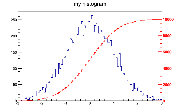
void twoscales() {
   TCanvas *c1 = new TCanvas("c1","different scales hists",600,400);
   //create, fill and draw h1
   gStyle->SetOptStat(kFALSE);
   TH1F *h1 = new TH1F("h1","my histogram",100,-3,3);
   for (Int_t i=0;i<10000;i++) h1->Fill(gRandom->Gaus(0,1));
   h1->Draw();
   c1->Update();
   //create hint1 filled with the bins integral of h1
   TH1F *hint1 = new TH1F("hint1","h1 bins integral",100,-3,3);
   Float_t sum = 0;
   for (Int_t i=1;i<=100;i++) {
      sum += h1->GetBinContent(i);
      hint1->SetBinContent(i,sum);
   }
   //scale hint1 to the pad coordinates
   Float_t rightmax = 1.1*hint1->GetMaximum();
   Float_t scale    = gPad->GetUymax()/rightmax;
   hint1->SetLineColor(kRed);
   hint1->Scale(scale);
   hint1->Draw("same");
   //draw an axis on the right side
   TGaxis*axis = new TGaxis(gPad->GetUxmax(),gPad->GetUymin(),
                            gPad->GetUxmax(),gPad->GetUymax(),
                            0,rightmax,510,"+L");
   axis->SetLineColor(kRed);
   axis->SetLabelColor(kRed);
   axis->Draw();
}By default, a histogram drawing includes the statistics box. Use TH1::SetStats(kFALSE) to eliminate the statistics box. If the statistics box is drawn, gStyle->SetOptStat(mode) allow you to select the type of displayed information . The parameter mode has up to nine digits that can be set OFF (0) or ON as follows:
mode = ksiourmen (default =000001111)
n = 1 the name of histogram is printede = 1 the number of entriesm = 1 the mean valuem = 2 the mean and mean error valuesr = 1 the root mean square (RMS)r = 2 the RMS and RMS erroru = 1 the number of underflowso = 1 the number of overflowsi = 1 the integral of binss = 1 the skewnesss = 2 the skewness and the skewness errork = 1 the kurtosisk = 2 the kurtosis and the kurtosis errorNever call SetOptStat(0001111) , but SetOptStat(1111) , because 0001111 will be taken as an octal number.
The method TStyle::SetOptStat(Option_t*option) can also be called with a character string as a parameter. The parameter option can contain:
n for printing the name of histograme the number of entriesm the mean valueM the mean and mean error valuesr the root mean square (RMS)R the RMS and RMS erroru the number of underflowso the number of overflowsi the integral of binss the skewnessS the skewness and the skewness errork the kurtosisK the kurtosis and the kurtosis error gStyle->SetOptStat("ne"); // prints the histogram name and number
// of entries
gStyle->SetOptStat("n"); // prints the histogram name
gStyle->SetOptStat("nemr"); // the default valueWith the option "same", the statistic box is not redrawn. With the option "sames", it is re-drawn. If it hides the previous statistics box, you can change its position with the next lines (where h is the histogram pointer):
root[] TPaveStats *s =
            (TPaveStats*)h->GetListOfFunctions()->FindObject("stats");
root[] s->SetX1NDC (newx1); // new x start position
root[] s->SetX2NDC (newx2); // new x end positionThe histogram classes inherit from the attribute classes: TAttLine, TAttFill, TAttMarker and TAttText. See the description of these classes for the list of options.
The TPad::SetTicks() method specifies the type of tick marks on the axis. Let tx=gPad->GetTickx() and ty=gPad->GetTicky().
tx = 1; tick marks on top side are drawn (inside)tx = 2; tick marks and labels on top side are drawnty = 1; tick marks on right side are drawn (inside)ty = 2; tick marks and labels on right side are drawntx=ty=0 by default only the left Y axis and X bottom axis are drawnUse TPad::SetTicks(tx,ty) to set these options. See also the methods of TAxis that set specific axis attributes. If multiple color-filled histograms are drawn on the same pad, the fill area may hide the axis tick marks. One can force the axis redrawing over all the histograms by calling:
Because the axis title is an attribute of the axis, you have to get the axis first and then call TAxis::SetTitle.
   h->GetXaxis()->SetTitle("X axis title");
   h->GetYaxis()->SetTitle("Y axis title");
   h->GetZaxis()->SetTitle("Z axis title");
The histogram title and the axis titles can be any TLatex string. The titles are part of the persistent histogram. For example if you wanted to write E with a subscript (T) you could use this:
For a complete explanation of the Latex mathematical expressions, see “Graphics and the Graphical User Interface”. It is also possible to specify the histogram title and the axis titles at creation time. These titles can be given in the “title” parameter. They must be separated by “;”:
Any title can be omitted:
The method SetTitle has the same syntax:
Like for any other ROOT object derived from TObject , the Clone method can be used. This makes an identical copy of the original histogram including all associated errors and functions:
   TH1F *hnew = (TH1F*)h->Clone(); // renaming is recommended,
   hnew->SetName("hnew");          // because otherwise you will have
                                   // two histograms with the same
// nameYou can scale a histogram ( TH1 *h ) such that the bins integral is equal to the normalization parameter norm:
The following statements create a ROOT file and store a histogram on the file. Because TH1 derives from TNamed , the key identifier on the file is the histogram name:
   TFile f("histos.root","new");
   TH1F h1("hgaus","histo from a gaussian",100,-3,3);
   h1.FillRandom("gaus",10000);
   h1->Write();
To read this histogram in another ROOT session, do:
One can save all histograms in memory to the file by:
For a more detailed explanation, see “Input/Output”.
TH1::KolmogorovTest( TH1* h2,Option_t *option) is statistical test of compatibility in shape between two histograms. The parameter option is a character string that specifies:
“U” include Underflows in test (also for 2-dim)
“O” include Overflows (also valid for 2-dim)
“N” include comparison of normalizations
“D” put out a line of “Debug” printout
“M” return the maximum Kolmogorov distance instead of prob
“X” run the pseudo experiments post-processor with the following procedure: it makes pseudo experiments based on random values from the parent distribution and compare the KS distance of the pseudo experiment to the parent distribution. Bin the KS distances in a histogram, and then take the integral of all the KS values above the value obtained from the original data to Monte Carlo distribution. The number of pseudo-experiments NEXPT is currently fixed at 1000. The function returns the integral. Note that this option “X” is much slower.
TH1::Smooth - smoothes the bin contents of a 1D histogram.
TH1::Integral(Option_t *opt)-returns the integral of bin contents in a given bin range. If the option “width” is specified, the integral is the sum of the bin contents multiplied by the bin width in x .
TH1::GetMean(int axis) - returns the mean value along axis.
TH1::GetStdDev(int axis) - returns the sigma distribution along axis.
TH1::GetRMS(int axis) - returns the Root Mean Square along axis.
TH1::GetEntries() - returns the number of entries.
TH1::GetAsymmetry(TH1 *h2,Double_t c2,Double_tdc2)
h2, where the asymmetry is defined as:1D , 2D , etc. histograms. The parameter c2 is an optional argument that gives a relative weight between the two histograms, and dc 2 is the error on this weight. This is useful, for example, when forming an asymmetry between two histograms from two different data sets that need to be normalized to each other in some way. The function calculates the errors assuming Poisson statistics on h1 and h2 (that is, dh=sqrt(h)). In the next example we assume that h1 and h2 are already filled:Then h3 is created and filled with the asymmetry between h1 and h2 ; h1 and h2 are left intact.
Note that the user’s responsibility is to manage the created histograms.
TH1::Reset() - resets the bin contents and errors of a histogram
GetMean, GetStdDev, etc.)By default, histogram statistics are computed at fill time using the unbinned data used to update the bin content. This means the values returned by GetMean, GetStdDev, etc., are those of the dataset used to fill the histogram, not those of the binned content of the histogram itself, unless one of the axes has been zoomed. (See the documentation on TH1::GetStats().) This is useful if you want to keep track of the mean and standard deviation of the dataset you are visualizing with the histogram, but it can lead to some unintuitive results.
For example, suppose you have a histogram with one bin between 0 and 100, then you fill it with a Gaussian dataset with mean 20 and standard deviation 2:
Right now, h->GetMean() will return 20 and h->GetStdDev() will return 2; ROOT calculated these values as we filled h. Next, zoom in on the Gaussian:
Now, h->GetMean() will return 50 and h->GetStdDev() will return 0. What happened? Well, GetMean and GetStdDev (and many other TH1 functions) return the statistics for bins in range; this is because the histogram only stores the contents of its bins, not the coordinates of the values used to fill it. So even though h has only one bin and it’s still included in the range, ROOT returns the binned statistics because SetRangeUser set the bit TAxis::kAxisRange to 1. This remains true even if you zoom out:
still results in GetMean and GetStdDev returning 50 and 0, respectively, because, even though this is the original range of the histogram, the X axis has still been assigned a range. To mark the X axis as having no range, you can call
without arguments or with arguments (0, 0). This sets the bit TAxis::kAxisRange to 0, and ROOT again uses the statistics calculated at fill time: GetMean and GetStdDev now return 20 and 2, respectively.
If you want ROOT to consistently return the statistics of the binned dataset stored in the histogram and not those of the dataset used to fill it, you can call TH1::ResetStats. This will delete the statistics originally calculated at fill time and replace them with those calculated from the bins; note that you cannot later retrieve the original statistics–they are lost. Continuing the example above,
results in GetMean and GetStdDev returning 50 and 0, respectively. If you fill the histogram again, the statistics will be a mix of binned and unbinned:
results in GetMean and GetStdDev returning 67.5 and 17.5, respectively; you must call TH1::ResetStats again to get consistent binned statistics.
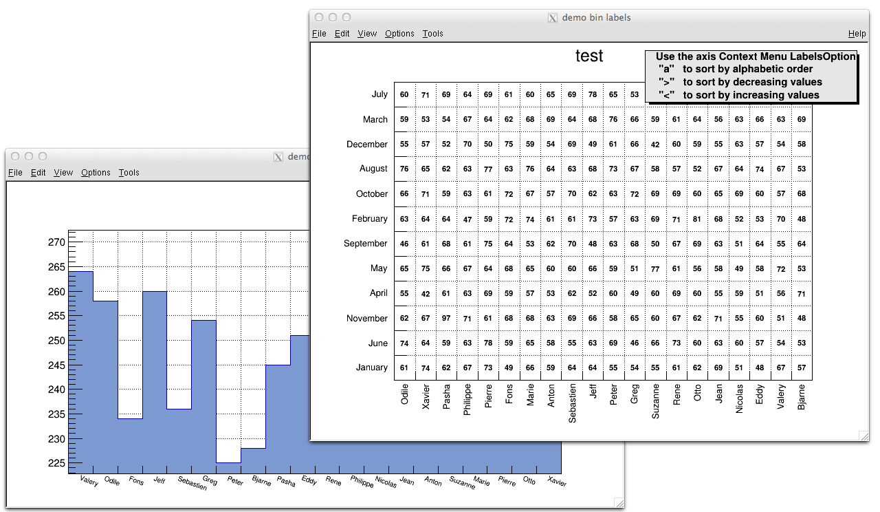
By default, a histogram axis is drawn with its numeric bin labels. One can specify alphanumeric labels instead.
To set an alphanumeric bin label call:
This can always be done before or after filling. Bin labels will be automatically drawn with the histogram.
See example in $ROOTSYS/tutorials/hist/hlabels1.C , hlabels2.C
You can also call a Fill() function with one of the arguments being a string:
hist1->Fill(somename,weigth);
hist2->Fill(x,somename,weight);
hist2->Fill(somename,y,weight);
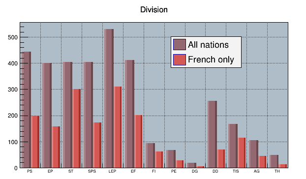
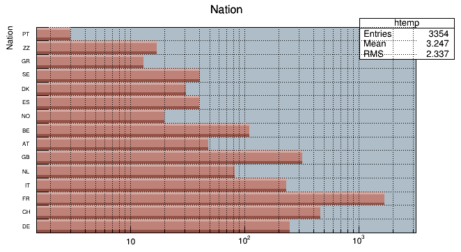
hist2->Fill(somenamex,somenamey,weight);You can use a char* variable type to histogram strings with TTree::Draw().
   // here "Nation" and "Division" are two char* branches of a Tree
   tree.Draw("Nation::Division", "", "text");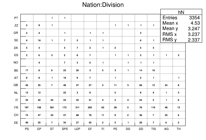
There is an example in $ROOTSYS/tutorials/io/tree/tree502_cernstaff.C.
If a variable is defined as char* it is drawn as a string by default. You change that and draw the value of char[0] as an integer by adding an arithmetic operation to the expression as shown below.
When using the options 2 or 3 above, the labels are automatically added to the list (THashList) of labels for a given axis. By default, an axis is drawn with the order of bins corresponding to the filling sequence. It is possible to reorder the axis alphabetically or by increasing or decreasing values. The reordering can be triggered via the TAxis context menu by selecting the menu item “LabelsOption” or by calling directly.
Here axis may be X, Y, or Z. The parameter option may be:
a” sort by alphabetic order>” sort by decreasing values<” sort by increasing valuesh” draw labels horizontalv” draw labels verticalu” draw labels up (end of label right adjusted)d” draw labels down (start of label left adjusted)When using the option second above, new labels are added by doubling the current number of bins in case one label does not exist yet. When the filling is terminated, it is possible to trim the number of bins to match the number of active labels by calling:
Here axis may be X, Y, or Z. This operation is automatic when using TTree::Draw . Once bin labels have been created, they become persistent if the histogram is written to a file or when generating the C++ code via SavePrimitive .
A THStack is a collection of TH1 (or derived) objects. Use THStack::Add( TH1 *h) to add a histogram to the stack. The THStack does not own the objects in the list.

By default, THStack::Draw draws the histograms stacked as shown in the left pad in the picture above. If the option "nostack" is used, the histograms are superimposed as if they were drawn one at a time using the "same" draw option . The right pad in this picture illustrates the THStack drawn with the "nostack" option.
Next is a simple example, for a more complex one see $ROOTSYS/tutorials/hist/hstack.C.
{
   THStack hs("hs","test stacked histograms");
   TH1F *h1 = new TH1F("h1","test hstack",100,-4,4);
   h1->FillRandom("gaus",20000);
   h1->SetFillColor(kRed);
   hs.Add(h1);
   TH1F *h2 = new TH1F("h2","test hstack",100,-4,4);
   h2->FillRandom("gaus",15000);
   h2->SetFillColor(kBlue);
   hs.Add(h2);
   TH1F *h3 = new TH1F("h3","test hstack",100,-4,4);
   h3->FillRandom("gaus",10000);
   h3->SetFillColor(kGreen);
   hs.Add(h3);
   TCanvas c1("c1","stacked hists",10,10,700,900);
   c1.Divide (1,2);
   c1.cd(1);
   hs.Draw();
   c1.cd(2);
   hs->Draw("nostack");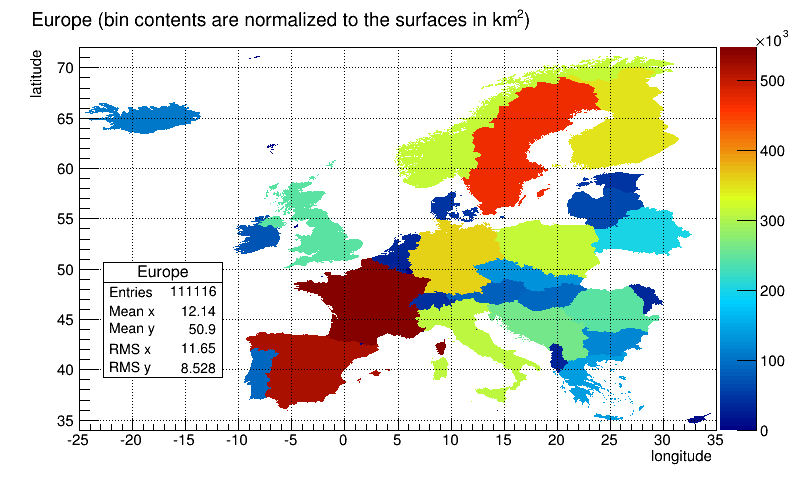
}TH2Poly is a 2D Histogram class allowing to define polygonal bins of arbitrary shape.
Each bin in the TH2Poly histogram is a TH2PolyBin object. TH2PolyBin is a very simple class containing the vertices and contents of the polygonal bin as well as several related functions.
Bins are defined using one of the AddBin() methods. The bin definition should be done before filling.
The following very simple macro shows how to build and fill a TH2Poly:
{
   TH2Poly *h2p = new TH2Poly();
   Double_t x1[] = {0, 5, 5};
   Double_t y1[] = {0, 0, 5};
   Double_t x2[] = {0, -1, -1, 0};
   Double_t y2[] = {0, 0, -1, -1};
   Double_t x3[] = {4, 3, 0, 1, 2.4};
   Double_t y3[] = {4, 3.7, 1, 4.7, 3.5};
   h2p->AddBin(3, x1, y1);
   h2p->AddBin(3, x2, y2);
   h2p->AddBin(3, x3, y3);
   h2p->Fill( 3, 1, 3);      // fill bin 1
   h2p->Fill(-0.5, -0.5, 7); // fill bin 2
   h2p->Fill(-0.7, -0.5, 1); // fill bin 2
   h2p->Fill( 1, 3, 5);      // fill bin 3
}
More examples can bin found in $ROOTSYS/tutorials/hist/th2poly*.C
Profile histograms are in many cases an elegant replacement of two-dimensional histograms. The relationship of two quantities X and Y can be visualized by a two-dimensional histogram or a scatter-plot; its representation is not particularly satisfactory, except for sparse data. If Y is an unknown [but single-valued] function of X, it can be displayed by a profile histogram with much better precision than by a scatter-plot. Profile histograms display the mean value of Y and its RMS for each bin in X. The following shows the contents [capital letters] and the values shown in the graphics [small letters] of the elements for bin j. When you fill a profile histogram with TProfile.Fill(x,y) :
H[j] will contain for each bin j the sum of the y values for this bin
L[j] contains the number of entries in the bin j
e[j] or s[j] will be the resulting error depending on the selected option. See “Build Options”.
E[j] = sum Y**2
L[j] = number of entries in bin J
H[j] = sum Y
h[j] = H[j] / L[j]
s[j] = sqrt[E[j] / L[j] - h[j]**2]
e[j] = s[j] / sqrt[L[j]]
In the special case where s[j] is zero, when there is only one entry per bin, e[j] is computed from the average of the s[j] for all bins. This approximation is used to keep the bin during a fit operation. The TProfile constructor takes up to eight arguments. The first five parameters are similar to TH1D constructor.
TProfile(const char *name,const char *title,Int_t nbinsx,
         Double_t xlow, Double_t xup, Double_t ylow, Double_t yup,
         Option_t *option)
All values of y are accepted at filling time. To fill a profile histogram, you must use TProfile::Fill function. Note that when filling the profile histogram the method TProfile::Fill checks if the variable y is between fYmin and fYmax. If a minimum or maximum value is set for the Y scale before filling, then all values below ylow or above yup will be discarded. Setting the minimum or maximum value for the Y scale before filling has the same effect as calling the special TProfile constructor above where ylow and yup are specified.
The last parameter is the build option. If a bin has N data points all with the same value Y, which is the case when dealing with integers, the spread in Y for that bin is zero, and the uncertainty assigned is also zero, and the bin is ignored in making subsequent fits. If SQRT(Y) was the correct error in the case above, then SQRT(Y)/SQRT(N) would be the correct error here. In fact, any bin with non-zero number of entries N but with zero spread (spread = s[j]) should have an uncertainty SQRT(Y)/SQRT(N). Now, is SQRT(Y)/SQRT(N) really the correct uncertainty ? That it is only in the case where the Y variable is some sort of counting statistics, following a Poisson distribution. This is the default case. However, Y can be any variable from an original NTUPLE, and does not necessarily follow a Poisson distribution. The computation of errors is based on Y = values of data points; N = number of data points.
' ' - the default is blank, the errors are:
spread/SQRT(N) for a non-zero spread
SQRT(Y)/SQRT(N) for a spread of zero and some data points
0 for no data points
‘ s ’ - errors are:
spread for a non-zero spread
SQRT(Y) for a Spread of zero and some data points
0 for no data points
‘ i ’ - errors are:
spread/SQRT(N) for a non-zero spread
1/SQRT(12*N) for a Spread of zero and some data points
0 for no data points
‘ G ’ - errors are:
spread/SQRT(N) for a non-zero spread
sigma/SQRT(N) for a spread of zero and some data points
0 for no data points
The option ’ i ’ is used for integer Y values with the uncertainty of \(\pm 0.5\), assuming the probability that Y takes any value between Y-0.5 and Y+0.5 is uniform (the same argument for Y uniformly distributed between Y and Y+1). An example is an ADC measurement. The ‘G’ option is useful, if all Y variables are distributed according to some known Gaussian of standard deviation Sigma. For example when all Y’s are experimental quantities measured with the same instrument with precision Sigma. The next figure shows the graphic output of this simple example of a profile histogram.
{
   // Create a canvas giving the coordinates and the size
   TCanvas *c1 = new TCanvas("c1", "Profile example",200,10,700,500);

   // Create a profile with the name, title, the number of bins,
   // the low and high limit of the x-axis and the low and high
   // limit of the y-axis.
   // No option is given so the default is used.
   hprof = new TProfile("hprof",
                        "Profile of pz versus px",100,-4,4,0,20);

   // Fill the profile 25000 times with random numbers
   Float_t px, py, pz;
   for ( Int_t i=0; i<25000; i++) {
      // Use the random number generator to get two numbers following
      // a gaussian distribution with mean=0 and sigma=1
      gRandom->Rannor(px,py);
      pz = px*px + py*py;
      hprof->Fill(px,pz,1);
   }
   hprof->Draw();
}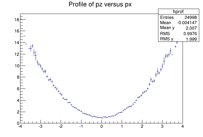
To draw a profile histogram and not show the error bars use the “HIST” option in the TProfile::Draw method. This will draw the outline of the TProfile.
You can make a profile from a histogram using the methods TH2::ProfileX and TH2::ProfileY.
To create a regular histogram from a profile histogram, use the method TProfile::ProjectionX .This example instantiates a TH1D object by copying the TH1D piece of TProfile.
You can do the same with a 2D profile using the method TProfile2D::ProjectionXY .
The 'prof' and 'profs' options in the TTree::Draw method generate a profile histogram ( TProfile ), given a two dimensional expression in the tree, or a TProfile2D given a three dimensional expression. See “Trees”. Note that you can specify 'prof' or 'profs' : 'prof' generates a TProfile with error on the mean, 'profs' generates a TProfile with error on the spread.
The class for a 2D Profile is called TProfile2D . It is in many cases an elegant replacement of a three-dimensional histogram. The relationship of three measured quantities X, Y and Z can be visualized by a three-dimensional histogram or scatter-plot; its representation is not particularly satisfactory, except for sparse data. If Z is an unknown (but single-valued) function of (X,Y), it can be displayed with a TProfile2D with better precision than by a scatter-plot. A TProfile2D displays the mean value of Z and its RMS for each cell in X, Y. The following shows the cumulated contents (capital letters) and the values displayed (small letters) of the elements for cell i,j.
When you fill a profile histogram with TProfile2D.Fill(x,y,z):
E[i,j] contains for each bin i,j the sum of the z values for this bin
L[i,j] contains the number of entries in the bin j
e[j] or s[j] will be the resulting error depending on the selected option. See “Build Options”.
E[i,j] = sum z
L[i,j] = sum l
h[i,j] = H[i,j ] / L[i,j]
s[i,j] = sqrt[E[i,j] / L[i,j]- h[i,j]**2]
e[i,j] = s[i,j] / sqrt[L[i,j]]
In the special case where s[i,j] is zero, when there is only one entry per cell, e[i,j] is computed from the average of the s[i,j] for all cells. This approximation is used to keep the cell during a fit operation.
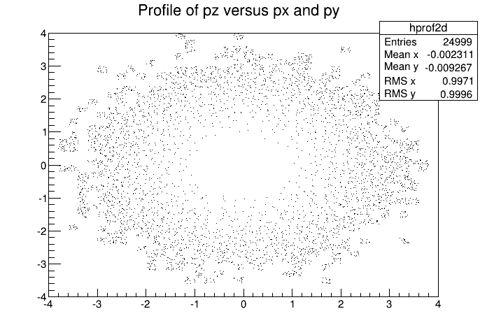
{
   // Creating a Canvas and a TProfile2D
   TCanvas *c1 = new TCanvas("c1",
                             "Profile histogram example",
                              200, 10,700,500);
   hprof2d = new TProfile2D("hprof2d",
                            "Profile of pz versus px and py",
                             40,-4,4,40,-4,4,0,20);

   // Filling the TProfile2D with 25000 points
   Float_t px, py, pz;
   for (Int_t i=0; i<25000; i++) {
      gRandom->Rannor(px,py);
      pz = px*px + py*py;
      hprof2d->Fill(px,py,pz,1);
   }
   hprof2d->Draw();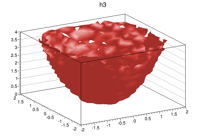
}Paint one Gouraud shaded 3d iso surface though a 3d histogram at the value computed as follow: SumOfWeights/(NbinsX*NbinsY*NbinsZ).
void hist3d() {
   TH3D *h3 = new TH3D("h3", "h3", 20, -2, 2, 20, -2, 2, 20, 0, 4);
   Double_t x,y,z;
   for (Int_t i=0; i<10000; i++) {
      gRandom->
      Rannor(x,y);
      z=x*x+y*y;
      h3->Fill(x,y,z);
   }
   h3->Draw("iso");
}
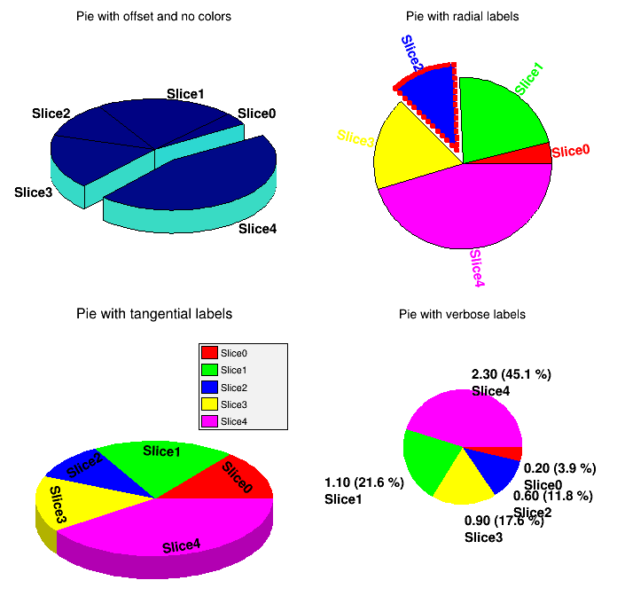
The TPie class allows to create a Pie Chart representation of a one dimensional data set. The data can come from an array of Double_t (or Float_t ) or from a 1D-histogram. The possible options to draw a TPie are:
“R” Paint the labels along the central “R”adius of slices.
“T” Paint the labels in a direction “T”angent to circle that describes the TPie.
“3D” Draw the pie-chart with a pseudo 3D effect.
“NOL” No OutLine: do not draw the slices’ outlines; any property over the slices’ line is ignored.
The method SetLabelFormat() is used to customize the label format. The format string must contain one of these modifiers:
%txt : to print the text label associated with the slice%val : to print the numeric value of the slice%frac : to print the relative fraction of this slice%perc : to print the % of this sliceSee the macro $ROOTSYS/tutorials/visualisation/graphics/piechart.C .
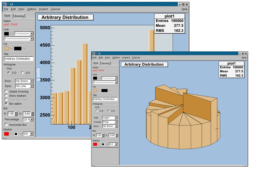
The classes T H1 Editor and T H2 Editor provides the user interface for setting histogram’s attributes and rebinning interactively.
sets the title of the histogram.
draw a 2D or 3D plot; according to the dimension, different drawing possibilities can be set.
add different error bars to the histogram (no errors, simple, etc.).
further things which can be added to the histogram (None, simple/smooth line, fill area, etc.)
draw a simple histogram without errors (= “HIST” draw option). In combination with some other draw options an outer line is drawn on top of the histogram
draw a marker on to of each bin (=“P” draw option).
draw a bar chart (=“B” draw option).
draw a bar chart (=“BAR” draw option); if selected, it will show an additional interface elements for bars: width, offset, percentage and the possibility to draw horizontal bars.
set histogram type Lego-Plot or Surface draw (Lego, Lego1.2, Surf, Surf1…5).
set the coordinate system (Cartesian, Spheric, etc.).
same as for 2D plot.
set the bar attributes: width and offset.
draw a horizontal bar chart.
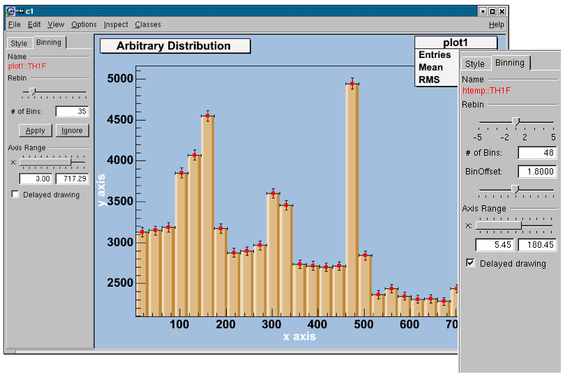
The binning tab has two different layouts. One is for a histogram, which is not drawn from an ntuple. The other one is available for a histogram, which is drawn from an ntuple. In this case, the rebin algorithm can create a rebinned histogram from the original data i.e. the ntuple.
To see the differences do:
   TFile f("hsimple.root");
   hpx->Draw("BAR1"); // non ntuple histogram
ntuple->Draw("px");// ntuple histogramRebin with a slider and the number of bins (shown in the field below the slider). The number of bins can be changed to any number, which divides the number of bins of the original histogram. A click on the Apply button will delete the origin histogram and will replace it by the rebinned one on the screen. A click on the Ignore button will restore the origin histogram.
with the slider, the number of bins can be enlarged by a factor of 2, 3, 4, 5 (moving to the right) or reduced by a factor of \(\frac{1}{2}\), \(\frac{1}{3}\), \(\frac{1}{4}\), \(\frac{1}{5}\).
the origin of the histogram can be changed within one binwidth. Using this slider the effect of binning the data into bins can be made visible (statistical fluctuations).
with a double slider it is possible to zoom into the specified axis range. It is also possible to set the upper and lower limit in fields below the slider.
all the Binning sliders can set to delay draw mode. Then the changes on the histogram are only updated, when the Slider is released. This should be activated if the redrawing of the histogram is time consuming.
set the title of the histogram
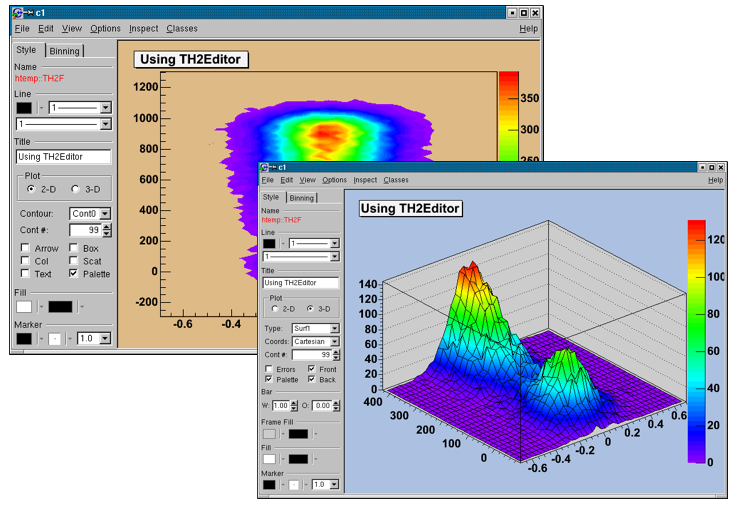
change the draw options of the histogram.
draw a 2D or 3D plot of the histogram; according to the dimension, the drawing possibilities are different.
draw a contour plot (None, Cont0…5)
set the number of Contours;
set the arrow mode and shows the gradient between adjacent cells;
a box is drawn for each cell with a color scale varying with contents;
draw bin contents as text;
a box is drawn for each cell with surface proportional to contents;
draw a scatter-plot (default);
the color palette is drawn.
set histogram type to Lego or surface plot; draw (Lego, Lego1.2, Surf, Surf1…5)
set the coordinate system (Cartesian, Spheric, etc.);
set the number of Contours (for e.g. Lego2 draw option);
draw errors in a Cartesian lego plot;
draw the color palette;
draw the front box of a Cartesian lego plot;
draw the back box of a Cartesian lego plot;
change the bar attributes: the width and offset.
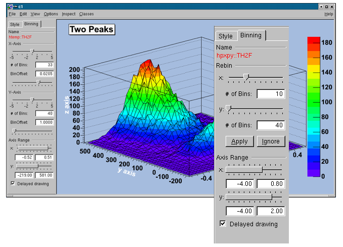
The Rebinning tab has two different layouts. One is for a histogram that is not drawn from an ntuple; the other one is available for a histogram, which is drawn from an ntuple. In this case, the rebin algorithm can create a rebinned histogram from the original data i.e. the ntuple. To see the differences do for example:
   TFile f ("hsimple.root");
   hpxpy->Draw("Lego2"); // non ntuple histogram
ntuple->Draw("px:py","","Lego2"); // ntuple histogramRebin with sliders (one for the x, one for the y-axis) and the number of bins (shown in the field below them can be changed to any number, which divides the number of bins of the original histogram. Selecting the Apply button will delete the origin histogram and will replace it by the rebinned one on the screen. Selecting the Ignore the origin histogram will be restored.
with the sliders the number of bins can be enlarged by a factor of 2,3,4,5 (moving to the right) or reduced by a factor of \(\frac{1}{2}\), \(\frac{1}{3}\), \(\frac{1}{4}\), \(\frac{1}{5}\).
with the BinOffset slider the origin of the histogram can be changed within one binwidth. Using this slider the effect of binning the data into bins can be made visible (=> statistical fluctuations).
with a double slider that gives the possibility for zooming. It is also possible to set the upper and lower limit in fields below the slider.
all the binning sliders can be set to delay draw mode. Then the changes on the histogram are only updated, when the Slider is released. This should be activated if the redrawing of the histogram is too time consuming.