WARNING: This documentation is not maintained anymore. Some part might be obsolete or wrong, some part might be missing but still some valuable information can be found there. Instead please refer to the ROOT Reference Guide and the ROOT Manual. If you think some information should be imported in the ROOT Reference Guide or in the ROOT Manual, please post your request to the ROOT Forum or via a Github Issue.
% Chapter: Math Libraries ________________________________________________________________________________________ WARNING: This documentation is not maintained anymore. Some part might be obsolete or wrong, some part might be missing but still some valuable information can be found there. Instead please refer to the ROOT Reference Guide and the ROOT Manual. If you think some information should be imported in the ROOT Reference Guide or in the ROOT Manual, please post your request to the ROOT Forum or via a Github Issue.
% Chapter: Math Libraries ________________________________________________________________________________________ WARNING: This documentation is not maintained anymore. Some part might be obsolete or wrong, some part might be missing but still some valuable information can be found there. Instead please refer to the ROOT Reference Guide and the ROOT Manual. If you think some information should be imported in the ROOT Reference Guide or in the ROOT Manual, please post your request to the ROOT Forum or via a Github Issue.
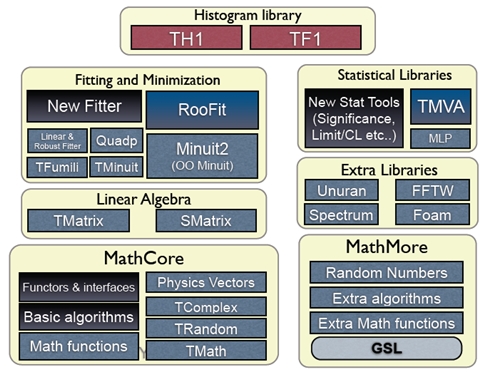
The aim of Math libraries in ROOT is to provide and to support a coherent set of mathematical and statistical functions. The latest developments have been concentrated in providing first versions of the MathCore and MathMore libraries, included in ROOT v5.08. Other recent developments include the new version of MINUIT, which has been re-designed and re-implemented in the C++ language. It is integrated in ROOT. In addition, an optimized package for describing small matrices and vector with fixed sizes and their operation has been developed (SMatrix). The structure is shown in the following picture.
MathCore provides a collection of functions and C++ classes for numerical computing. This library includes only the basic mathematical functions and algorithms and not all the functionality required by the physics community. A more advanced mathematical functionality is provided by the MathMore library. The current set of included classes, which are provided in the ROOT::Math namespace are:
Basic special functions like the gamma, beta and error function.
Mathematical functions used in statistics, such as the probability density functions and the cumulative distributions functions (lower and upper integral of the pdf’s).
Generic function classes and interfaces for evaluating one-dimensional (ROOT::Math::IBaseFunctiononeDim) and multi-dimensional functions (ROOT::Math::IBaseFunctionMultiDim) and parametric function interfaces for evaluating functions with parameters in one (ROOT::Math::IParametricFunctionOneDim) or multi dimensions (ROOT::Math::IParametricFunctionMultiDim). A set of user convenient wrapper classes, such as ROOT::Math::Functor is provided for wrapping user-classes in the needed interface, required to use the algorithms of the ROOT Mathematical libraries.
ROOT::Math::Minimizer interface)Fitting classes: set of classes for fitting generic data sets. These classes are provided in the namespace ROOT::Fit. They are describing separately in the Fitting chapter.
The sets described above is independent of ROOT libraries and can be built as a set of standalone classes. In addition MathCore provides the following classes (depending on ROOT libCore library):
TMath: namespace with mathematical functions and basic function algorithms.TComplex: class for complex numbers.TRandom and the derived classes TRandom1, TRandom2 and TRandom3, implementing the pseudo-random number generators.A detailed description for all MathCore classes is available in the Doxygen online reference documentation.
The MathMore library provides an advanced collection of functions and C++ classes for numerical computing. This is an extension of the functionality provided by the MathCore library. The MathMore library is implemented wrapping in C++ the GNU Scientific Library (GSL). The current set, provided in the ROOT::Math namespace include:
Special mathematical functions (like Bessel functions, Legendre polynomials, etc.. )
Additional mathematical functions used in statistics such as probability density functions, cumulative distributions functions and their inverse which are not in MathCore but present in the GSL library.
Numerical algorithms for one dimensional functions based on implementation of the GNU Scientific Library (GSL):
Numerical integration classes implementing the interface ROOT::Math::Integrator which is based on the Adaptive integration algorithms of QUADPACK
Numerical differentiation via ROOT::Math::GSLDerivator
Root finder implementing the ROOT::Math::RootFinder interface, using different solver algorithms from GSL
one-dimensional Minimization implementing the interfaceROOT::Math::IMinimizer1D
Interpolation via ROOT::Math::Interpolation. All the GSL interpolation types are supported
Function approximation based on Chebyshev polynomials via the class ROOT::Math::Chebyshev
Random number generators and distributions based on GSL using the ROOT::Math::Random<Engine_type> class.
Polynomial evaluation and root solvers
The mathematical functions are implemented as a set of free functions in the namespace ROOT::Math. The naming used for the special functions is the same proposed for the C++ standard (see C++ standard extension proposal document).The MathMore library is implemented wrapping in C++ the GNU Scientific Library ( MathMore requires a version of GSL larger or equal 1.8. The source code of MathMore is distributed under the GNU General Public License.
MathMore (and its ROOT Cling dictionary) can be built within ROOT whenever a GSL library is found in the system. The GSL library and header file location can be specified in the ROOT configure script, by doing:
./configure --with-gsl-incdir=... --with-gsl-libdir=...MathMore can be built also a stand-alone library (without requiring ROOT) downloding the tar file from the Web at this link. In this case the library will not contain the dictionary information and therefore cannot be used interactively
More information on the classes and functions present in MathMore is available in the online reference documentation.
In the namespace, TMath, a collection of free functions is provided for the following functionality:
numerical constants (like pi, e, h, etc.);
trigonometric and elementary mathematical functions;
functions to work with arrays and collections (e.g. functions to find min and max of arrays);
statistic functions to work on array of data (e.g. mean and RMS of arrays);
algorithms for binary search/hashing sorting;
special mathematical functions like Bessel, Erf, Gamma, etc.;
statistical functions, like common probability and cumulative (quantile) distributions
geometrical functions.
For more details, see the reference documentation of TMath at <http://root.cern.ch/root/htmldoc/TMath.html>.
TMath offers a wide range of constants in the form of inline functions. Notice that they are not defined as C/C++ preprocessor macros. This set of functions includes one or more definitions for the following constants:
A set of miscellaneous elementary mathematical functions is provided along with a set of basic trigonometrical functions. Some of this functions refer to basic mathematical functions like the square root, the power to a number of the calculus of a logarithm, while others are used for number treatment, like rounding.
Although there are some functions that are not in the standard C math library (like Factorial), most of the functionality offered here is just a wrapper of the first ones. Nevertheless, some of the them also offer some security checks or a better precision, like the trigonometrical functions ASin(x), ACos(x) or ATan(x).
 // Generate a vector with 10 random numbers
 vector<double> v(10);
 std::generate(v.begin(), v.end(), rand);

 // Find the minimum value of the vector (iterator version)
 vector<double>::iterator it;
 it = TMath::LocMin(v.begin(), v.end());
 std::cout << *it << std::endl;

 // The same with the old-style version
 int i;
 i = TMath::LocMin(10, &v[0]);
 std::cout << v[i] << std::endl;
Another example of these functions can be found in $ROOTSYS/tutorials/permute.C.
This set of functions processes arrays to calculate:
These functions, as the array algorithms, have two different interfaces. An old-style one where the size of the array is passed as a first argument followed by a pointer to the array itself and a modern C++-like interface that receives two iterators to it.
 // Size of the array
 const int n = 100;

 // Vector v with random values
 vector<double> v(n);
 std::generate(v.begin(), v.end(), rand);

 // Weight vector w
 vector<double> w(n);
 std::fill(w.begin(), w.end, 1);

 double mean;

 // Calculate the mean of the vector
 // with iterators
 mean = TMath::Mean(v.begin(), v.end());

 // old-style
 mean = TMath::Mean(n, &v[0]);

 // Calculate the mean with a weight vector
 // with iterators
 mean = TMath::Mean(v.begin(), v.end(), w.begin());

 // old-style
mean = TMath::Mean(n, &v[0], &w[0]);TMath also provides special functions like Bessel, Error functions, Gamma or similar plus statistical mathematical functions, including probability density functions, cumulative distribution and their inverse.
The majority of the special functions and the statistical distributions are provided also as free functions in the ROOT::Math namespace. See one of the next paragraph for the complete description of the functions provided in ROOT::Math. The user is encourage to use those versions of the algorithms rather than the ones in TMath.
Functions not present in ROOT::Math and provided only by TMath are:
The example tutorial GammaFun.C and mathBeta.C in $ROOTSYS/tutorials shows an example of use of the ROOT::Math special functions
In ROOT pseudo-random numbers can be generated using the TRandom classes. 4 different types exist: TRandom, TRandom1, TRandom2 and TRandom3. All they implement a different type of random generators. TRandom is the base class used by others. It implements methods for generating random numbers according to pre-defined distributions, such as Gaussian or Poisson.
Pseudo-random numbers are generated using a linear congruential random generator. The multipliers used are the same of the BSD rand() random generator. Its sequence is:
\(x_{n+1} = (ax_n + c) mod m\) with \(a =1103515245\), \(c = 12345\) and \(m =2^{31}\).
This type of generator uses a state of only a 32 bit integer and it has a very short period, 231,about 109, which can be exhausted in just few seconds. The quality of this generator is therefore BAD and it is strongly recommended to NOT use for any statistical study.
This random number generator is based on the Ranlux engine, developed by M. Lüsher and implemented in Fortran by F. James. This engine has mathematically proven random proprieties and a long period of about 10171. Various luxury levels are provided (1,2,3,4) and can be specified by the user in the constructor. Higher the level, better random properties are obtained at a price of longer CPU time for generating a random number. The level 3 is the default, where any theoretical possible correlation has very small chance of being detected. This generator uses a state of 24 32-bits words. Its main disadvantage is that is much slower than the others (see timing table). For more information on the generator see the following article:
This generator is based on the maximally equi-distributed combined Tausworthe generator by L’Ecuyer. It uses only 3 32-bits words for the state and it has a period of about 1026. It is fast and given its small states, it is recommended for applications, which require a very small random number size. For more information on the generator see the following article:
This is based on the Mersenne and Twister pseudo-random number generator, developed in 1997 by Makoto Matsumoto and Takuji Nishimura. The newer implementation is used, referred in the literature as MT19937. It is a very fast and very high quality generator with a very long period of 106000. The disadvantage of this generator is that it uses a state of 624 words. For more information on the generator see the following article:
TRandom3 is the recommended random number generator, and it is used by default in ROOT using the global gRandom object (see chapter gRandom).
The seeds for the generators can be set in the constructor or by using the SetSeed method. When no value is given the generator default seed is used, like 4357 for TRandom3. In this case identical sequence will be generated every time the application is run. When the 0 value is used as seed, then a unique seed is generated using a TUUID, for TRandom1, TRandom2 and TRandom3. For TRandom the seed is generated using only the machine clock, which has a resolution of about 1 sec. Therefore identical sequences will be generated if the elapsed time is less than a second.
The method Rndm() is used for generating a pseudo-random number distributed between 0 and 1 as shown in the following example:
   // use default seed
   // (same random numbers will be generated each time)
   TRandom3 r; // generate a number in interval ]0,1] (0 is excluded)
   r.Rndm();
   double x[100];
   r.RndmArray(100,x); // generate an array of random numbers in ]0,1]
   TRandom3 rdm(111);      // construct with a user-defined seed
   // use 0: a unique seed will be automatically generated using TUUID
   TRandom1 r1(0);
   TRandom2 r2(0);
   TRandom3 r3(0);
   // seed generated using machine clock (different every second)
TRandom r0(0);The TRandom base class provides functions, which can be used by all the other derived classes for generating random variates according to predefined distributions. In the simplest cases, like in the case of the exponential distribution, the non-uniform random number is obtained by applying appropriate transformations. In the more complicated cases, random variates are obtained using acceptance-rejection methods, which require several random numbers.
TRandom3 r;
   // generate a gaussian distributed number with:
   // mu=0, sigma=1 (default values)
   double x1 = r.Gaus();
   double x2 = r.Gaus(10,3);    // use mu = 10, sigma = 3;
The following table shows the various distributions that can be generated using methods of the TRandom classes. More information is available in the reference documentation for TRandom. In addition, random numbers distributed according to a user defined function, in a limited interval, or to a user defined histogram, can be generated in a very efficient way using TF1::GetRandom() or TH1::GetRandom().
| Distributions | Description |
Double_t Uniform(Double_t x1,Double_t x2 ) |
Uniform random numbers between x1,x2 |
Double_t Gaus(Double_t mu,Double_t sigma ) |
Gaussian random numbers. Default values: |
Double_t Exp(Double_t tau) |
Exponential random numbers with mean tau. |
Double_t Landau(Double_t mean,Double_t s igma) |
Landau distributed random numbers. Default values: |
|
Breit-Wigner distributed random numbers. Default values |
|
Poisson random numbers |
Int_t Binomial(Int_t ntot,Double_t prob ) |
Binomial Random numbers |
Circle(Double_t &x,Double_t &y,Double_t r) |
Generate a random 2D point a circle of radius |
|
Generate a random 3D point a sphere of radius |
Rannor(Double_t &a,Double_t &b) |
Generate a pair of Gaussian random numbers with |
An interface to a new package, UNU.RAN, (Universal Non Uniform Random number generator for generating non-uniform pseudo-random numbers) was introduced in ROOT v5.16.
UNU.RAN is an ANSI C library licensed under GPL. It contains universal (also called automatic or black-box) algorithms that can generate random numbers from large classes of continuous (in one or multi-dimensions), discrete distributions, empirical distributions (like histograms) and also from practically all standard distributions. An extensive online documentation is available at the UNU.RAN Web Site http://statmath.wu-wien.ac.at/unuran/
The ROOT class TUnuran is used to interface the UNURAN package. It can be used as following:
   TUnuran unr;
   // initialize unuran to generate normal random numbers using
   // a "arou" method
   unr.Init("normal()","method=arou");
   ...
   // sample distributions N times (generate N random numbers)
   for (int i = 0; i<N; ++i)
double x = unr.Sample();TUnuranContDist that can be created for example from a TF1 function providing the pdf (probability density function) . The user can optionally provide additional information via TUnuranContDist::SetDomain(min,max) like the domain() for generating numbers in a restricted region. // 1D case: create a distribution from two TF1 object
// pointers pdfFunc
TUnuranContDist dist( pdfFunc);
// initialize unuran passing the distribution and a string
// defining the method
unr.Init(dist, "method=hinv");
// sample distribution N times (generate N random numbers)
for (int i = 0; i < N; ++i)
double x = unr.Sample();TUnuranMultiContDist, which can be created from a the multi-dimensional pdf. // Multi- dimensional case from a TF1 (TF2 or TF3) objects
TUnuranMultiContDist dist( pdfFuncMulti);
// the recommended method for multi-dimensional function is "hitro"
unr.Init(dist,"method=hitro");
// sample distribution N times (generate N random numbers)
double x[NDIM];
for (int i = 0; i<N; ++i)
unr.SampleMulti(x);TUnuranDiscrDist, which can be initialized from a TF1 or from a vector of probabilities. // Create distribution from a vector of probabilities
double pv[NSize] = {0.1,0.2,...};
TUnuranDiscrDist dist(pv,pv+NSize);
// the recommended method for discrete distribution is
unr.Init(dist, "method=dgt");
// sample N times (generate N random numbers)
for (int i = 0; i < N; ++i)
int k = unr.SampleDiscr();TUnuranEmpDist. In this case one can generate random numbers from a set of un-bin or bin data. In the first case the parent distribution is estimated by UNU.RAN using a gaussian kernel smoothing algorithm. The TUnuranEmpDist distribution class can be created from a vector of data or from TH1 (using the bins or from its buffer for un-binned data). // Create distribution from a set of data
// vdata is an std::vector containing the data
TUnuranEmpDist dist(vdata.begin(),vdata.end());
unr.Init(dist);
// sample N times (generate N random numbers)
for (int i = 0; i<N; ++i)
double x = unr.Sample();Poisson and Binomial, one can use directly a function in the TUnuran class. This is more convenient in passing distribution parameters than using directly the string interface. TUnuran unr;
// Initialize unuran to generate normal random numbers from the
// Poisson distribution with parameter mu
unr.InitPoisson(mu);
...
// Sample distributions N times (generate N random numbers)
for (int i = 0; i<N; ++i)
int k = unr.SampleDiscr();Functionality is also provided via the C++ classes for using a different random number generator by passing a TRandom pointer when constructing the TUnuran class (by default the ROOT gRandom is passed to UNURAN).
Here are the CPU times obtained using the four random classes on an lxplus machine with an Intel 64 bit architecture and compiled using gcc 3.4:
TRandom (ns/call) |
TRandom1 (ns/call) |
TRandom2 (ns/call) |
TRandom3 (ns/call) |
|
Rndm() |
6 | 9 | ||
Gaus() |
31 | 161 | 35 | 42 |
Rannor() |
116 | 216 | 126 | 130 |
Poisson(m-10) |
147 | 1161 | 162 | 239 |
Poisson(m=10) UNURAN |
80 | 294 | 89 | 99 |
The mathematical functions are present in both MathCore and MathMore libraries. All mathematical functions are implemented as free functions in the namespace ROOT::Math. The most used functions are in the MathCore library while the others are in the MathMore library. The functions in MathMore are all using the implementation of the GNU Scientific Library (GSL). The naming of the special functions is the same defined in the C++ Technical Report on Standard Library extensions. The special functions are defined in the header file Math/SpecFunc.h.
ROOT::Math::beta(double x,double y) -evaluates the beta function: \[B(x,y) = \frac{\Gamma(x) \Gamma(y)}{\Gamma(x+y)}\]
double ROOT::Math::erf(double x) - evaluates the error function encountered in integrating the normal distribution: \[erf(x) = \frac{2}{\sqrt{\pi}} \int_{0}^{x} e^{-t^2} dt\]
double ROOT::Math::erfc(double x) - evaluates the complementary error function: \[erfc(x) = 1 - erf(x) = \frac{2}{\sqrt{\pi}} \int_{x}^{\infty} e^{-t^2} dt\]
double ROOT::Math::tgamma(double x) - calculates the gamma function: \[\Gamma(x) = \int_{0}^{\infty} t^{x-1} e^{-t} dt\]
double ROOT::Math::assoc_legendre(unsigned l,unsigned m,double x) -computes the associated Legendre polynomials (with m>=0, l>=m and |x|<1): \[P_{l}^{m}(x) = (1-x^2)^{m/2} \frac{d^m}{dx^m} P_{l}(x)\]
double ROOT::Math::comp_ellint_1(double k) - calculates the complete elliptic integral of the first kind (with \(0 \le k^2 \le 1\): \[
K(k) = F(k, \pi / 2) = \int_{0}^{\pi /2} \frac{d \theta}{\sqrt{1 - k^2 \sin^2{\theta}}}
\]
double ROOT::Math::comp_ellint_2(double k) - calculates the complete elliptic integral of the second kind (with \(0 \le k^2 \le 1\)): \[
E(k) = E(k , \pi / 2) = \int_{0}^{\pi /2} \sqrt{1 - k^2 \sin^2{\theta}} d \theta
\]
double ROOT::Math::comp_ellint_3(double n,double k) - calculates the complete elliptic integral of the third kind (with \(0 \le k^2 \le 1\)): \[
\Pi (n, k, \pi / 2) = \int_{0}^{\pi /2} \frac{d \theta}{(1 - n \sin^2{\theta})\sqrt{1 - k^2 \sin^2{\theta}}}
\]
double ROOT::Math::conf_hyperg(double a,double b,double z) - calculates the confluent hyper-geometric functions of the first kind: \[
_{1}F_{1}(a;b;z) = \frac{\Gamma(b)}{\Gamma(a)} \sum_{n=0}^{\infty} \frac{\Gamma(a+n)}{\Gamma(b+n)} \frac{z^n}{n!}
\]
double ROOT::Math::conf_hypergU(double a,double b,double z) - calculates the confluent hyper-geometric functions of the second kind, known also as Kummer function of the second type. It is related to the confluent hyper-geometric function of the first kind: \[
U(a,b,z) = \frac{ \pi}{ \sin{\pi b } } \left[ \frac{ _{1}F_{1}(a,b,z) } {\Gamma(a-b+1) } - \frac{ z^{1-b} { _{1}F_{1}}(a-b+1,2-b,z)}{\Gamma(a)} \right]
\]
double ROOT::Math::cyl_bessel_i(double nu,double x) - calculates the modified Bessel function of the first kind, also called regular modified (cylindrical) Bessel function: \[
I_{\nu} (x) = i^{-\nu} J_{\nu}(ix) = \sum_{k=0}^{\infty} \frac{(\frac{1}{2}x)^{\nu + 2k}}{k! \Gamma(\nu + k + 1)}
\]
double ROOT::Math::cyl_bessel_j(double nu,double x) - calculates the (cylindrical) Bessel function of the first kind, also called regular (cylindrical) Bessel function: \[
J_{\nu} (x) = \sum_{k=0}^{\infty} \frac{(-1)^k(\frac{1}{2}x)^{\nu + 2k}}{k! \Gamma(\nu + k + 1)}
\]
double ROOT::Math::cyl_bessel_k(double nu,double x) - calculates the modified Bessel function of the second kind, also called irregular modified (cylindrical) Bessel function for \(x > 0\), \(v > 0\): \[
K_{\nu} (x) = \frac{\pi}{2} i^{\nu + 1} (J_{\nu} (ix) + iN(ix)) = \left\{ \begin{array}{cl} \frac{\pi}{2} \frac{I_{-\nu}(x) - I_{\nu}(x)}{\sin{\nu \pi}} & \mbox{for non-integral $\nu$} \\ \frac{\pi}{2} \lim{\mu \to \nu} \frac{I_{-\mu}(x) - I_{\mu}(x)}{\sin{\mu \pi}} & \mbox{for integral $\nu$} \end{array} \right.
\]
double ROOT::Math::cyl_neumann(double nu,double x) - calculates the (cylindrical) Bessel function of the second kind, also called irregular (cylindrical) Bessel function or (cylindrical) Neumann function: \[
N_{\nu} (x) = Y_{\nu} (x) = \left\{ \begin{array}{cl} \frac{J_{\nu} \cos{\nu \pi}-J_{-\nu}(x)}{\sin{\nu \pi}} & \mbox{for non-integral $\nu$} \\ \lim{\mu \to \nu} \frac{J_{\mu} \cos{\mu \pi}-J_{-\mu}(x)}{\sin{\mu \pi}} & \mbox{for integral $\nu$} \end{array} \right.
\]
double ROOT::Math::ellint_1(double k,double phi) - calculates incomplete elliptic integral of the first kind (with \(0 \le k^2 \le 1\)): \[
K(k) = F(k, \pi / 2) = \int_{0}^{\pi /2} \frac{d \theta}{\sqrt{1 - k^2 \sin^2{\theta}}}
\]
double ROOT::Math::ellint_2(double k,double phi) - calculates the complete elliptic integral of the second kind (with \(0 \le k^2 \le 1\)): \[
E(k) = E(k , \pi / 2) = \int_{0}^{\pi /2} \sqrt{1 - k^2 \sin^2{\theta}} d \theta
\]
double ROOT::Math::ellint_3(double n,double k,double phi) - calculates the complete elliptic integral of the third kind (with \(0 \le k^2 \le 1\)): \[
\Pi (n, k, \pi / 2) = \int_{0}^{\pi /2} \frac{d \theta}{(1 - n \sin^2{\theta})\sqrt{1 - k^2 \sin^2{\theta}}}
\]
double ROOT::Math::expint(double x) - calculates the exponential integral: \[
Ei(x) = - \int_{-x}^{\infty} \frac{e^{-t}}{t} dt
\]
double ROOT::Math::hyperg(double a,double b,double c,double x) - calculates Gauss’ hyper-geometric function: \[
_{2}F_{1}(a,b;c;x) = \frac{\Gamma(c)}{\Gamma(a) \Gamma(b)} \sum_{n=0}^{\infty} \frac{\Gamma(a+n)\Gamma(b+n)}{\Gamma(c+n)} \frac{x^n}{n!}
\]
double ROOT::Math::legendre(unsigned l,double x) - calculates the Legendre polynomials for \(l \ge 0\), \(|x| \le 1\) in the Rodrigues representation: \[
P_{l}(x) = \frac{1}{2^l l!} \frac{d^l}{dx^l} (x^2 - 1)^l
\]
double ROOT::Math::riemann_zeta(double x) - calculates the Riemann zeta function: \[
\zeta (x) = \left\{ \begin{array}{cl} \sum_{k=1}^{\infty}k^{-x} & \mbox{for $x > 1$} \\ 2^x \pi^{x-1} \sin{(\frac{1}{2}\pi x)} \Gamma(1-x) \zeta (1-x) & \mbox{for $x < 1$} \end{array} \right.
\]
double ROOT::Math::sph_bessel(unsigned n,double x) - calculates the spherical Bessel functions of the first kind (also called regular spherical Bessel functions): \[
j_{n}(x) = \sqrt{\frac{\pi}{2x}} J_{n+1/2}(x)
\]
double ROOT::Math::sph_neumann(unsigned n,double x) - calculates the spherical Bessel functions of the second kind (also called irregular spherical Bessel functions or spherical Neumann functions): \[
n_n(x) = y_n(x) = \sqrt{\frac{\pi}{2x}} N_{n+1/2}(x)
\]
Probability density functions of various distributions. All the functions, apart from the discrete ones, have the extra location parameter x0, which by default is zero. For example, in the case of a gaussian pdf, x0 is the mean, mu, of the distribution. All the probability density functions are defined in the header file Math/DistFunc.h and are part of the MathCore libraries. The definition of these functions is documented in the reference doc for statistical functions:
double ROOT::Math::beta_pdf(double x,double a, double b);
double ROOT::Math::binomial_pdf(unsigned int k,double p,unsigned int n);
double ROOT::Math::breitwigner_pdf(double x,double gamma,double x0=0);
double ROOT::Math::cauchy_pdf(double x,double b=1,double x0=0);
double ROOT::Math::chisquared_pdf(double x,double r,double x0=0);
double ROOT::Math::exponential_pdf(double x,double lambda,double x0=0);
double ROOT::Math::fdistribution_pdf(double x,double n,double m,double x0=0);
double ROOT::Math::gamma_pdf(double x,double alpha,double theta,double x0=0);
double ROOT::Math::gaussian_pdf(double x,double sigma,double x0=0);
double ROOT::Math::landau_pdf(double x,double s,double x0=0);
double ROOT::Math::lognormal_pdf(double x,double m,double s,double x0=0);
double ROOT::Math::normal_pdf(double x,double sigma,double x0=0);
double ROOT::Math::poisson_pdf(unsigned int n,double mu);
double ROOT::Math::tdistribution_pdf(double x,double r,double x0=0);
double ROOT::Math::uniform_pdf(double x,double a,double b,double x0=0);For all the probability density functions, we have the corresponding cumulative distribution functions and their complements. The functions with extension _cdf calculate the lower tail integral of the probability density function:
\[ D(x) = \int_{-\infty}^{x} p(x') dx' \]
while those with the cdf_c extension calculate the upper tail of the probability density function, so-called in statistics the survival function. For example, the function:
evaluates the lower tail of the Gaussian distribution: \[ D(x) = \int_{-\infty}^{x} {\frac{1}{\sqrt{2 \pi \sigma^2}}} e^{-(x'-x_0)^2 / 2\sigma^2} dx' \]
while the function:
evaluates the upper tail of the Gaussian distribution: \[ D(x) = \int_{x}^{+\infty} {\frac{1}{\sqrt{2 \pi \sigma^2}}} e^{-(x'-x_0)^2 / 2\sigma^2} dx' \]
The cumulative distributions functions are defined in the header file Math/ProbFunc.h. The majority of the CDF’s are present in the MathCore, apart from the chisquared, fdistribution, gamma and tdistribution, which are in the MathMore library.
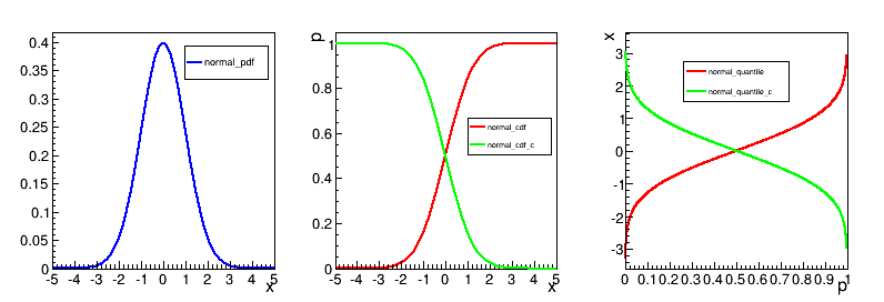
For almost all the cumulative distribution functions (_cdf) and their complements (_cdf_c) present in the library, we provide the inverse functions. The inverse of the cumulative distribution function is called in statistics quantile function. The functions with the extension _quantile calculate the inverse of the cumulative distribution function (lower tail integral of the probability density function), while those with the quantile_c extension calculate the inverse of the complement of the cumulative distribution (upper tail integral). All the inverse distributions are in the MathMore library and are defined in the header file Math/ProbFuncInv.h.
The following picture illustrates the available statistical functions (PDF, CDF and quantiles) in the case of the normal distribution.
ROOT provides C++ classes implementing numerical algorithms to solve a wide set of problem, like:
In order to use these algorithm the user needs to provide a function. ROOT provides a common way of specifying them via some interfaces
To get a consistency in the mathematical methods within ROOT, there exists a set of interfaces to define the basic behaviour of a mathematical function. In order to use the classes presented in this chapter, the mathematical functions defined by the user must inherit from any of the classes seen in the figure:
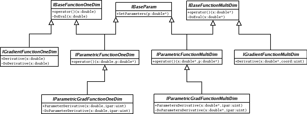
These interfaces are used for numerical algorithms operating only on one-dimensional functions and cannot be applied to multi-dimensional functions. For this case the users needs to define a function object which evaluates in one dimension, and the object will have to derivate from the following:
ROOT::Math::IBaseFunctionOneDim: This class is the most basic function. Provides a method to evaluate the function given a value (simple double) by implementing double operator() (const double ). The user class defined only needs to reimplement the pure abstract method double DoEval(double x), that will do the work of evaluating the function at point x.Example on how to create a class that represents a mathematical function. The user only has to override two methods from IBaseFunctionOneDim:
#include "Math/IFunction.h"

class MyFunction: public ROOT::Math::IBaseFunctionOneDim
{
   double DoEval(double x) const
   {
      return x*x;
   }

   ROOT::Math::IBaseFunctionOneDim* Clone() const
   {
      return new MyFunction();
   }
};ROOT::Math::IGradientFunctionOneDim: Some of the numerical algorithm will need to calculate the derivatives of the function. In these cases, the user will have to provide the necessary code for this to happen. The interface defined in IGradientFunctionOneDim introduced the method double Derivative(double x) that will return the derivative of the function at the point x. The class inherit by the user will have to implement the abstract method double DoDerivative(double x), leaving the rest of the class untouched.
Example for implementing a gradient one-dimensional function:
#include "Math/IFunction.h"

class MyGradientFunction: public ROOT::Math::IGradientFunctionOneDim
{
public:
   double DoEval(double x) const
   {
      return sin(x);
   }

   ROOT::Math::IBaseFunctionOneDim* Clone() const
   {
      return new MyGradientFunction();
   }

   double DoDerivative(double x) const
   {
      return -cos(x);
   }

};The most generic case of a multidimensional function has similar approach. Some examples will be shown next. It is important to notice, that one dimensional functions can be also implemented through the interfaces that will be presented here. Nevertheless, the user needs to implement those following the indications of the previous chapter, for algorithm working exclusivly on one-dimensional functions. For algorithms working on both one-dimensional and multi-dimensional functions they should instead use this interface.
ROOT::Math::IBaseFunctionMultiDim: This interface provides the double operator() (const double*) that takes an array of doubles with all the values for the different dimensions. In this case, the user has to provide the functionality for two different functions: double DoEval(const double*) and unsigned int NDim(). The first ones evaluates the function given the array that represents the multiple variables. The second returns the number of dimensions of the function.
Example of implementing a basic multi-dimensional function:
#include "Math/IFunction.h"

class MyFunction: public ROOT::Math::IBaseFunctionMultiDim
{
public:
   double DoEval(const double* x) const
   {
      return x[0] + sin(x[1]);
   }

   unsigned int NDim() const
   {
      return 2;
   }

   ROOT::Math::IBaseFunctionMultiDim* Clone() const
   {
      return new MyFunction();
   }

};ROOT::Math::IGradientFunctionMultiDim: This interface offers the same functionality as the base function plus the calculation of the derivative. It only adds the double Derivative(double* x, uint ivar) method for the user to implement. This method must implement the derivative of the function with respect to the variable indicated with the second parameter.Example of implementing a multi-dimensional gradient function
#include "Math/IFunction.h"

class MyGradientFunction: public ROOT::Math::IGradientFunctionMultiDim
{
public:
   double DoEval(const double* x) const
   {
      return x[0] + sin(x[1]);
   }

   unsigned int NDim() const
   {
      return 2;
   }

   ROOT::Math::IGradientFunctionMultiDim* Clone() const
   {
      return new MyGradientFunction();
   }

   double DoDerivative(const double* x, unsigned int ipar) const
   {
      if ( ipar == 0 )
         return sin(x[1]);
      else
         return x[0] + x[1] * cos(x[1]);
   }

};These interfaces, for evaluating multi-dimensional functions are used for fitting. These interfaces are defined in the header file Math/IParamFunction.h. See also the documentation of the ROOT::Fit classes in the Fitting chapter for more information.
ROOT::Math::IParametricFunctionMultiDim: Describes a multi dimensional parametric function. Similarly to the one dimensional version, the user needs to provide the method void SetParameters(double* p) as well as the getter methods const double * Parameters() and uint NPar(). Example of creating a parametric function:#include "Math/IFunction.h"
#include "Math/IParamFunction.h"
class MyParametricFunction: public ROOT::Math::IParametricFunctionMultiDim
{
private:
const double* pars;
public:
double DoEvalPar(const double* x, const double* p) const
{
return p[0] * x[0] + sin(x[1]) + p[1];
}
unsigned int NDim() const
{
return 2;
}
ROOT::Math::IParametricFunctionMultiDim* Clone() const
{
return new MyParametricFunction();
}
const double* Parameters() const
{
return pars;
}
void SetParameters(const double* p)
{
pars = p;
}
unsigned int NPar() const
{
return 2;
}
};ROOT::Math::IParametricGradFunctionMultiDim: Provides an interface for parametric gradient multi-dimensional functions. In addition to function evaluation it provides the gradient with respect to the parameters, via the method ParameterGradient(). This interface is only used in case of some dedicated fitting algorithms, when is required or more efficient to provide derivatives with respect to the parameters. Here is an example:#include "Math/IFunction.h"
#include "Math/IParamFunction.h"
class MyParametricGradFunction:
public ROOT::Math::IParametricGradFunctionMultiDim
{
private:
const double* pars;
public:
double DoEvalPar(const double* x, const double* p) const
{
return p[0] * x[0] + sin(x[1]) + p[1];
}
unsigned int NDim() const
{
return 2;
}
ROOT::Math::IParametricGradFunctionMultiDim* Clone() const
{
return new MyParametricGradFunction();
}
const double* Parameters() const
{
return pars;
}
void SetParameters(const double* p)
{
pars = p;
}
unsigned int NPar() const
{
return 2;
}
double DoParameterDerivative(const double* x, const double* p,
unsigned int ipar) const
{
if ( ipar == 0 )
return sin(x[1]) + p[1];
else
return p[0] * x[0] + x[1] * cos(x[1]) + p[1];
}
};To facilitate the user to insert their own type of function in the needed function interface, helper classes, wrapping the user interface in the ROOT::Math function interfaces are provided. this will avoid the user to re-implement dedicated function classes, following the code example shown in the previous paragraphs.
There is one possible wrapper for every interface explained in the previous section. The following table indicates the wrapper for the most basic ones:
| Interface | Function Wrapper |
|---|---|
ROOT::Math::IBaseFunctionOneDim |
ROOT::Math::Functor1D |
ROOT::Math::IGradientFunctionOneDim |
ROOT::Math::GradFunctor1D |
ROOT::Math::IBaseFunctionMultiDim |
ROOT::Math::Functor |
ROOT::Math::IGradientFunctionMultiDim |
ROOT::Math::GradFunctor |
Thee functor wrapper are defined in the header file Math/Functor.h.
The ROOT::Math::Functor1D is used to wrap one-dimensional functions It can wrap all the following types: * A free C function of type double ()(double ). * Any C++ callable object implementation double operator()( double ). * A class member function with the correct signature like double Foo::Eval(double ). In this case one pass the object pointer and a pointer to the member function (&Foo::Eval).
Example:
#include "Math/Functor.h"

class MyFunction1D {

public:

   double operator()(double x) const {
      return x*x;
   }

   double Eval(double x) const { return x+x; }
};

double freeFunction1D(double  x ) {
   return 2*x;
}

int main()
{
   // wrapping a free function
   ROOT::Math::Functor1D  f1(&freeFunction1D);

   MyFunction1D myf1;

   // wrapping a function object implementing operator()
   ROOT::Math::Functor1D  f2(myf1);

   // wrapping a class member function
   ROOT::Math::Functor1D f3(&myf1,&MyFunction1D::Eval);

   cout << f1(2) << endl;
   cout << f2(2) << endl;
   cout << f3(2) << endl;

   return 0;
}The ROOT::Math::GradFunctor1D class is used to wrap one-dimensional gradient functions. It can be constructed in three different ways: * Any object implementing both double operator()( double) for the function evaluation and double Derivative(double) for the function derivative. * Any object implementing any member function like Foo::XXX(double ) for the function evaluation and any other member function like Foo::YYY(double ) for the derivative. * Any two function objects implementing double operator()( double ) . One object provides the function evaluation, the other the derivative. One or both function object can be a free C function of type double ()(double ).
The class ROOT::Math::Functor is used to wrap in a very simple and convenient way multi-dimensional function objects. It can wrap all the following types: * Any C++ callable object implementing double operator()( const double * ). * A free C function of type double ()(const double * ). * A member function with the correct signature like Foo::Eval(const double * ). In this case one pass the object pointer and a pointer to the member function (&Foo::Eval).
The function dimension is required when constructing the functor.
Example of using Functor:
#include "Math/Functor.h"

class MyFunction {

public:
   double operator()(const double *x) const {
      return x[0]+x[1];
   }

   double Eval(const double * x) const { return x[0]+x[1]; }
};

double freeFunction(const double * x )
{
   return x[0]+x[1];
}

int main()
{
   // test directly calling the function object
   MyFunction myf;

   // test from a free function pointer
   ROOT::Math::Functor f1(&freeFunction,2);

   // test from function object
   ROOT::Math::Functor f2(myf,2);

   // test from a member function
   ROOT::Math::Functor f3(&myf,&MyFunction::Eval,2);

   double x[] = {1,2};

   cout << f1(x) << endl;
   cout << f2(x) << endl;
   cout << f3(x) << endl;

   return 0;
}The class ROOT::Math::GradFunctor is used to wrap in a very C++ callable object to make gradient functions. It can be constructed in three different way: * From an object implementing both double operator()( const double * ) for the function evaluation and double Derivative(const double *, int icoord) for the partial derivatives. * From an object implementing any member function like Foo::XXX(const double *) for the function evaluation and any member function like Foo::XXX(const double *, int icoord) for the partial derivatives. * From an function object implementing double operator()( const double * ) for the function evaluation and another function object implementing double operator() (const double *, int icoord) for the partial derivatives.
The function dimension is required when constructing the functor.
In many cases, the user works with the TF1 class. The mathematical library in ROOT provides some solutions to wrap these into the interfaces needed by other methods. If the desired interface to wrap is one-dimensional, the class to use is ROOT::Math::WrappedTF1. The default constructor takes a TF1 reference as an argument, that will be wrapped with the interfaces of a ROOT::Math::IParametricGradFunctionOneDim. Example:
#include "TF1.h"
#include "Math/WrappedTF1.h"

int main()
{

   TF1 f("Sin Function", "sin(x)+y",0,3);

   ROOT::Math::WrappedTF1 wf1(f);

   cout << f(1) << endl;
   cout << wf1(1) << endl;

   return 0;
}
For a TF1 defining a multidimensional function or in case we need to wrap in a multi-dimensional function interface, the class to use is ROOT::Math::WrappedMultiTF1. Following the usual procedure, setting the TF1 though the constructor, will wrap it into a ROOT::Math::IParametricGradFunctionMultiDim. Example:
#include "TF1.h"
#include "Math/WrappedMultiTF1.h"

int main()
{

   TF2 f("Sin Function", "sin(x) + y",0,3,0,2);

   ROOT::Math::WrappedMultiTF1 wf1(f);

   double x[] = {1,2};

   cout << f(x) << endl;
   cout << wf1(x) << endl;

   return 0;
}The algorithms provided by ROOT for numerical integration are implemented following the hierarchy shown in the next image. ROOT::Math::VirtualIntegrator defines the most basic functionality while the specific behaviours for one or multiple dimensions are implemented in ROOT::Math::VirtualIntegratorOneDim and ROOT::Math::VirtualIntegratorMultiDim. These interfaces define the integrator functionality with abstract methods to set the function, to compute the integral or to set the integration tolerance. These methods must be implemented in the concrete classes existing for the different integration algorithms. The user cannot create directly these virtual integrator interfaces. He needs to create the ROOT::Math::IntegratorOneDim class for integrating one-dimensional functions and ROOT::Math::IntegratorMultiDim for multi-dimensional functions. Through the ROOT Plug-In Manager, the user can initialize ROOT::Math::IntegratorOneDim or ROOT::Math::IntegratorMultiDim with any of the concrete integration classes without dealing with them directly. These two classes provide the same interface as in VirtualIntegratorOneDim and VirtualIntegratorMultiDim, but with the possibility to choose in the constructor, which method will be used to perform the integration.
The method to set the function to be integrated, must be of the function interface type described before. ROOT::Math::IBaseFunctionOneDimFunction is used for ROOT::Math::IBaseFunctionMultiDim and The only difference between the ROOT::Math::IntegratorOneDim and ROOT::Math::IntegratorMultiDim resides in the dimensionality of that function and some specific that will be seen afterwards for the one dimensional one.
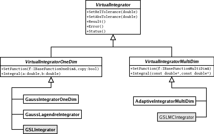
The rest of the classes shown above in the diagram are the specialized classes provided. Each one implements a different method that will be explained in detail. It is important to notice that the two grayed classes (the one which name starts by GSL) are part of the MathMore library. We will later show in more detail the differences between the implementations.
ROOT::Math::IntegratorOneDimHere is a code example on how to use the ROOT::Math::IntegratorOneDim class (note that the class is defined in the header file Math/Integrator.h). In this example we create different instance of the class using some of the available algorithms in ROOT. If no algorithm is specified, the default one is used. The default Integrator together with other integration options such as relative and absolute tolerance, can be specified using the static method of the ROOT::Math::IntegratorOneDimOptions
#include "Math/Integrator.h"

const double ERRORLIMIT = 1E-3;

double f(double x) {
   return x;
}

double f2(const double * x) {
   return x[0] + x[1];
}


int testIntegration1D() {

   const double RESULT = 0.5;
   int status = 0;

   // set default tolerances for all integrators
   ROOT::Math::IntegratorOneDimOptions::SetDefaultAbsTolerance(1.E-6);
   ROOT::Math::IntegratorOneDimOptions::SetDefaultRelTolerance(1.E-6);

   ROOT::Math::Functor1D wf(&f);
   ROOT::Math::Integrator ig(ROOT::Math::IntegrationOneDim::kADAPTIVESINGULAR);
   ig.SetFunction(wf);
   double val = ig.Integral(0,1);
   std::cout << "integral result is " << val << std::endl;
   status += std::fabs(val-RESULT) > ERRORLIMIT;

   ROOT::Math::Integrator ig2(ROOT::Math::IntegrationOneDim::kNONADAPTIVE);
   ig2.SetFunction(wf);
   val = ig2.Integral(0,1);
   std::cout << "integral result is " << val << std::endl;
   status += std::fabs(val-RESULT) > ERRORLIMIT;

   ROOT::Math::Integrator ig3(wf, ROOT::Math::IntegrationOneDim::kADAPTIVE);
   val = ig3.Integral(0,1);
   std::cout << "integral result is " << val << std::endl;
   status += std::fabs(val-RESULT) > ERRORLIMIT;

   ROOT::Math::Integrator ig4(ROOT::Math::IntegrationOneDim::kGAUSS);
   ig4.SetFunction(wf);
   val = ig4.Integral(0,1);
   std::cout << "integral result is " << val << std::endl;
   status += std::fabs(val-RESULT) > ERRORLIMIT;

   ROOT::Math::Integrator ig4(ROOT::Math::IntegrationOneDim::kLEGENDRE);
   ig4.SetFunction(wf);
   val = ig4.Integral(0,1);
   std::cout << "integral result is " << val << std::endl;
   status += std::fabs(val-RESULT) > ERRORLIMIT;

   return status;
}Here we provide a brief description of the different integration algorithms, which are also implemented as separate classes. The algorithms can be instantiated using the following enumeration values:
| Enumeration name | Integrator class |
|---|---|
ROOT::Math::IntegratorOneDim::kGAUSS |
ROOT::Math::GaussianIntegrator |
ROOT::Math::IntegratorOneDim::kLEGENDRE |
ROOT::Math:::GausLegendreIntegrator |
ROOT::Math::Integration::kNONADAPTIVE |
ROOT::Math:::GSLIntegrator |
ROOT::Math::Integration::kADAPTIVE |
ROOT::Math:::GSLIntegrator |
ROOT::Math::Integration::kADAPTIVESINGULAR |
ROOT::Math:::GSLIntegrator |
It uses the most basic Gaussian integration algorithm, it uses the 8-point and the 16-point Gaussian quadrature approximations. It is derived from the DGAUSS routine of the CERNLIB by S. Kolbig. This class Here is an example of using directly the GaussIntegrator class
#include "TF1.h"
#include "Math/WrappedTF1.h"
#include "Math/GaussIntegrator.h"

int main()
{
   TF1 f("Sin Function", "sin(x)", 0, TMath::Pi());
   ROOT::Math::WrappedTF1 wf1(f);

   ROOT::Math::GaussIntegrator ig;

   ig.SetFunction(wf1, false);
   ig.SetRelTolerance(0.001);

   cout << ig.Integral(0, TMath::PiOver2()) << endl;

   return 0;
}This class implementes the Gauss-Legendre quadrature formulas. This sort of numerical methods requieres that the user specifies the number of intermediate function points used in the calculation of the integral. It will automatically determine the coordinates and weights of such points before performing the integration. We can use the example above, but replacing the creation of a ROOT::Math::GaussIntegrator object with ROOT::Math::GaussLegendreIntegrator.
This is a wrapper for the QUADPACK integrator implemented in the GSL library. It supports several integration methods that can be chosen in construction time. The default type is adaptive integration with singularity applying a Gauss-Kronrod 21-point integration rule. For a detail description of the GSL methods visit the GSL user guide This class implements the best algorithms for numerical integration for one dimensional functions. We encourage the use it as the main option, bearing in mind that it uses code from the GSL library, wich is provided in the MathMore library of ROOT.
The interface to use is the same as above. We have now the possibility to specify a different integration algorithm in the constructor of the ROOT::Math::GSLIntegrator class.
// create the adaptive integrator with the 51 point rule
ROOT::Math::GSLIntegrator ig(ROOT::Math::Integration::kADAPTIVE, ROOT::Math::Integration::kGAUSS51);
ig.SetRelTolerance(1.E-6);  // set relative tolerance
ig.SetAbsTolerance(1.E-6);   // set absoulte tolerance
The algorithm is controlled by the given absolute and relative tolerance. The iterations are continued until the following condition is satisfied \[
absErr <= max ( epsAbs, epsRel * Integral)
\] Where absErr is an estimate of the absolute error (it can be retrieved with GSLIntegrator::Error()) and Integral is the estimate of the function integral (it can be obtained with GSLIntegrator::Result())
The possible integration algorithm types to use with the GSLIntegrator are the following. More information is provided in the GSL users documentation. * ROOT::Math::Integration::kNONADAPTIVE : based on gsl_integration_qng. It is a non-adaptive procedure which uses fixed Gauss-Kronrod-Patterson abscissae to sample the integrand at a maximum of 87 points. It is provided for fast integration of smooth functions. * ROOT::Math::Integration::kADAPTIVE: based on gsl_integration_qag. It is an adaptiva Gauss-Kronrod integration algorithm, the integration region is divided into subintervals, and on each iteration the subinterval with the largest estimated error is bisected. It is possible to specify the integration rule as an extra enumeration parameter. The possible rules are * Integration::kGAUSS15 : 15 points Gauss-Konrod rule (value = 1) * Integration::kGAUSS21 : 21 points Gauss-Konrod rule (value = 2) * Integration::kGAUSS31 : 31 points Gauss-Konrod rule (value = 3) * Integration::kGAUSS41 : 41 points Gauss-Konrod rule (value = 4) * Integration::kGAUSS51 : 51 points Gauss-Konrod rule (value = 5) * Integration::kGAUSS61 : 61 points Gauss-Konrod rule (value = 6) The higher-order rules give better accuracy for smooth functions, while lower-order rules save time when the function contains local difficulties, such as discontinuities. If no integration rule is passed, the 31 points rule is used as default.
ROOT::Math::Integration::kADAPTIVESINGULAR: based on gsl_integration_qags. It is an integration type which can be used in the case of the presence of singularities.It uses the Gauss-Kronrod 21-point integration rule. This is the default algorithmNote that when using the common ROOT::Math::IntegratorOneDIm class the enumeration type defining the algorithm must be defined in the namespace ROOT::Math::IntegrationOneDim (to distinguish from the multi-dimensional case) and the rule enumeration (or its corresponding integer) can be passed in the constructor of the ROOT::Math::IntegratorOneDIm.
The multi-dimensional integration algorithm should be applied to functions with dimension larger than one. Adaptive multi-dimensional integration works for low function dimension, while MC integration can be applied to higher dimensions.
ROOT::Math::IntegratorMultiDimHere is a code example on how to use the ROOT::Math::IntegratorOneDim class (note that the class is defined in the header file Math/Integrator.h). In this example we create different instance of the class using some of the available algorithms in ROOT.
#include "Math/IntegratorMultiDim.h"
#include "Math/Functor.h"


double f2(const double * x) {
   return x[0] + x[1];
}

int testIntegrationMultiDim() {

   const double RESULT = 1.0;
   const double ERRORLIMIT = 1E-3;
   int status = 0;

   ROOT::Math::Functor wf(&f2,2);
   double a[2] = {0,0};
   double b[2] = {1,1};

   ROOT::Math::IntegratorMultiDim ig(ROOT::Math::IntegrationMultiDim::kADAPTIVE);
   ig.SetFunction(wf);
   double val = ig.Integral(a,b);
   std::cout << "integral result is " << val << std::endl;
   status += std::fabs(val-RESULT) > ERRORLIMIT;

   ROOT::Math::IntegratorMultiDim ig2(ROOT::Math::IntegrationMultiDim::kVEGAS);
   ig2.SetFunction(wf);
   val = ig2.Integral(a,b);
   std::cout << "integral result is " << val << std::endl;
   status += std::fabs(val-RESULT) > ERRORLIMIT;

   ROOT::Math::IntegratorMultiDim ig3(wf,ROOT::Math::IntegrationMultiDim::kPLAIN);
   val = ig3.Integral(a,b);
   std::cout << "integral result is " << val << std::endl;
   status += std::fabs(val-RESULT) > ERRORLIMIT;

   ROOT::Math::IntegratorMultiDim ig4(wf,ROOT::Math::IntegrationMultiDim::kMISER);
   val = ig4.Integral(a,b);
   std::cout << "integral result is " << val << std::endl;
   status += std::fabs(val-RESULT) > ERRORLIMIT;

   return status;
}Here is the types, that can be specified as enumeration and the corresponding classes
| Enumeration name | Integrator class |
|---|---|
ROOT::Math::IntegratorMultiDim::kADAPTIVE |
ROOT::Math::AdaptiveIntegratorMultiDim |
ROOT::Math::IntegratorMultiDim::kVEGAS |
ROOT::Math:::GSLMCIntegrator |
ROOT::Math::IntegratorMultiDim::kMISER |
ROOT::Math:::GSLMCIntegrator |
ROOT::Math::IntegratorMultiDim::kPLAIN |
ROOT::Math:::GSLMCIntegrator |
The control parameters for the integration algorithms can be specified using the ROOT::Math::IntegratorMultiDimOptions class. Static methods are provided to change the default values. It is possible to print the list of default control parameters using the ROOT::Math::IntegratorMultiDimOptions::Print function. Example:
ROOT::Math::IntegratorMultiDimOptions opt;
opt.Print();
          Integrator Type :        ADAPTIVE
       Absolute tolerance :           1e-09
       Relative tolerance :           1e-09
           Workspace size :          100000
     (max) function calls :          100000
Depending on the algorithm, some of the control parameters might have no effect.
ROOT::Math::AdaptiveIntegratorMultiDimThis class implements an adaptive quadrature integration method for multi dimensional functions. It is described in this paper Genz, A.A. Malik, An adaptive algorithm for numerical integration over an N-dimensional rectangular region, J. Comput. Appl. Math. 6 (1980) 295-302. It is part of the MathCore library. The user can control the relative and absolute tolerance and the maximum allowed number of function evaluation.
ROOT::Math::GSLMCIntegratorIt is a class for performing numerical integration of a multidimensional function. It uses the numerical integration algorithms of GSL, which reimplements the algorithms used in the QUADPACK, a numerical integration package written in Fortran. Plain MC, MISER and VEGAS integration algorithms are supported for integration over finite (hypercubic) ranges. For a detail description of the GSL methods visit the GSL users guide. Specific configuration options (documented in the GSL user guide) for the ROOT::Math::GSLMCIntegration can be set directly in the class, or when using it via the ROOT::Math::IntegratorMultiDim interface, can be defined using the ROOT::Math::IntegratorMultiDimOptions.
There are in ROOT only two classes to perform numerical derivation. One of them is in the MathCore library while the other is in the MathMore wrapping an integration function from the GSL library. * RichardsonDerivator: Implements the Richardson method for numerical integration. It can calculate up to the third derivative of a function. * GSLDerivator of MathMore based on GSL.
The algorithms provided by ROOT for numerical integration are implemented following the hierarchy shown in the next image. The left branch of classes are used for one dimensional minimization, while the right one is used for multidimensional minimization. In the case of multidimensional minimization we have also the classes TMinuitMinimizer implemented using TMinuit, TFumiliMinimizer implemented using TFumili for least square or likelihood minimizations. We encourage the use of the GSL algorithms for one dimensional minimization and Minuit2 (or the old versionMinuit) for multi dimensional minimization.
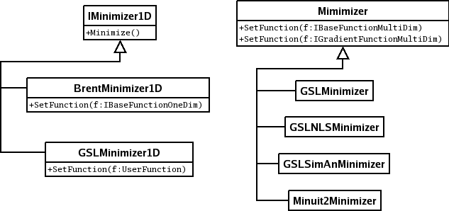
These algorithms are for finding the minimum of a one-dimensional minimization function. The function to minimize must be given to the class implementing the algorithm as a ROOT::Math::IBaseFunctionOneDim object. The algorithms supported are only bracketing algorithm which do not use derivatives information.
Two classes exist. One in the MathCore library implementing the Brent method (not using the derivatives) and one in the MathMore library implementing several different methods, using in some case the derivatives.
ROOT::Math::BrentMinimizer1DThis class implements the Brent method to minimize one-dimensional function. An interval containing the function minimum must be provided. Here is an example where we define the function to minimize as a lambda function (requires C++11). The function to minimize must be given to the class implementing the algorithm as a ROOT::Math::IBaseFunctionOneDim object.
  ROOT::Math::Functor1D func( [](double x){ return 1 + -4*x + 1*x*x; } );

   ROOT::Math::BrentMinimizer1D bm;
   bm.SetFunction(func, -10,10);
   bm.Minimize(10,0,0);
   cout << "Minimum: f(" << bm.XMinimum() << ") = " <<bm.FValMinimum() << endl;
Note that when setting the function to minimize, one needs to provide the interval range to find the minimum. In the Minimize call, the maximum number of function calls, the relative and absolute tolerance must be provided.
ROOT::Math::GSLMInimizer1DThis class wraps two different methods from the GSL. The algorithms which can be chosen at construction time are GOLDENSECTION, which is the simplest method but the slowest and BRENT (the default one) which combines the golden section with a parabolic interpolation. The algorithm can be chosen as a different enumeration in the constructor: * ROOT::Math::Minim1D::kBRENT for the Brent algorithm (default) * ROOT::Math::Minim1D::kGOLDENSECTION for the golden section algorithm
 // this makes class with the default Brent algorithm
 ROOT::Math::GSLMinimizer1D minBrent;
  // this make the class with the Golden Section algorithm
   ROOT::Math::GSLMinimizer1D minGold(ROOT::Math::Minim1D::kGOLDENSECTION);
The interface to set the function and to minimize is the same as in the case of the BrentMinimizer1D.
It is possible to perform the one-dimensional minimization/maximization of a function by using directly the function class in ROOT, TF1 of the Hist library. The minmization is implemented in TF1 using the BrentMInimizer1D and available with the class member functions * TF1::GetMinimum/TF1::GetMaximum to find the function minimum/maximum value * TF1::GetMinimumX/TF1::GetMaximumX to find the x value corresponding at the function minimum.
The interval to search for the minimum (the default is the TF1 range), tolerance and maximum iterations can be provided as optional parameters of the TF1::GetMinimum/Maximum functions.
All the algorithms for multi-dimensional minimization are implementing the ROOT::Math::Minimizer interface and they can be used in the same way and one can switch between minimizer at run-time. The minimizer concrete class can be in different ROOT libraries and they can be instantiate using the ROOT plug-in manager. More information on multi-dimensional minimization is provided in the Fitting Histogram chapter.
The function must be given to the class implementing the algorithm as a ROOT::Math::IBaseFunctionOneDim object. Some of the algorithm requires the derivatives of the function. In that case a ROOT::Math::IGradientFunctionOneDim object must be provided.
GenVector is a package intended to represent vectors and their operations and transformations, such as rotations and Lorentz transformations, in 3 and 4 dimensions. The 3D space is used to describe the geometry vectors and points, while the 4D space-time is used for physics vectors representing relativistic particles. These 3D and 4D vectors are different from vectors of the linear algebra package, which describe generic N-dimensional vectors. Similar functionality is currently provided by the CLHEP GenVector provides class templates for modeling the vectors. The user can control how the vector is internally represented. This is expressed by a choice of coordinate system, which is supplied as a template parameter when the vector is constructed. Furthermore, each coordinate system is itself a template, so that the user can specify the underlying scalar type.
The GenVector classes do not inherit from TObject, therefore cannot be used as in the case of the physics vector classes in ROOT collections.
In addition, to optimize performances, no virtual destructors are provided. In the following paragraphs, the main characteristics of GenVector are described. A more detailed description of all the GenVector classes is available also at http://seal.cern.ch/documents/mathlib/GenVector.pdf
We try to minimize any overhead in the run-time performance. We have deliberately avoided the use of any virtual function and even virtual destructors in the classes. In addition, as much as possible functions are defined as inline. For this reason, we have chosen to use template classes to implement the GenVector concepts instead of abstract or base classes and virtual functions. It is then recommended to avoid using the GenVector classes polymorphically and developing classes inheriting from them.
Mathematically vectors and points are two distinct concepts. They have different transformations, as vectors only rotate while points rotate and translate. You can add two vectors but not two points and the difference between two points is a vector. We then distinguish for the 3 dimensional case, between points and vectors, modeling them with different classes:
ROOT::Math::DisplacementVector2D and ROOT::Math::DisplacementVector3D template classes describing 2 and 3 component direction and magnitude vectors, not rooted at any particular point;
ROOT::Math::PositionVector2D and ROOT::Math::PositionVector3D template classes modeling the points in 2 and 3 dimensions.
For the 4D space-time vectors, we use the same class to model them, ROOT::Math::LorentzVector, since we have recognized a limited need for modeling the functionality of a 4D point.
The vector classes are based on a generic type of coordinate system, expressed as a template parameter of the class. Various classes exist to describe the various coordinates systems:
2D coordinate system classes:
ROOT::Math::Cartesian2D, based on (x,y);
ROOT::Math::Polar2D, based on (r,phi);
3D coordinate system classes:
ROOT::Math::Cartesian3D, based on (x,y,z);
ROOT::Math::Polar3D, based on (r,theta,phi);
ROOT::Math::Cylindrical3D, based on (rho,z,phi)
ROOT::Math::CylindricalEta3D, based on (rho,eta,phi), where eta is the pseudo-rapidity;
4D coordinate system classes:
ROOT::Math::PxPyPzE4D, based on based on (px,py,pz,E);
ROOT::Math::PxPyPzM4D, based on based on (px,py,pz,M);
ROOT::Math::PtEtaPhiE4D, based on based on (pt,eta,phi,E);
ROOT::Math::PtEtaPhiM4D, based on based on (pt,eta,phi,M);
Users can define the vectors according to the coordinate type, which is the most efficient for their use. Transformations between the various coordinate systems are available through copy constructors or the assignment (=) operator. For maximum flexibility and minimize memory allocation, the coordinate system classes are templated on the scalar type. To avoid exposing templated parameter to the users, typedefs are defined for all types of vectors based on doubles. See in the examples for all the possible types of vector classes, which can be constructed by users with the available coordinate system types.
The 2D and 3D points and vector classes can be associated to a tag defining the coordinate system. This can be used to distinguish between vectors of different coordinate systems like global or local vectors. The coordinate system tag is a template parameter of the ROOT::Math::DisplacementVector3D and ROOT::Math::PositionVector3D (and also for 2D classes). A default tag exists for users who do not need this functionality, ROOT::Math::DefaultCoordinateSystemTag.
The transformations are modeled using simple (non-template) classes, using double as the scalar type to avoid too large numerical errors. The transformations are grouped in rotations (in 3 dimensions), Lorentz transformations and Poincare transformations, which are translation/rotation combinations. Each group has several members which may model physically equivalent transformations but with different internal representations. Transformation classes can operate on all type of vectors by using the operator ()or the operator * and the transformations can be combined via the operator *. The available transformations are:
3D rotation classes
rotation described by a 3x3 matrix (ROOT::Math::Rotation3D)
rotation described by Euler angles (ROOT::Math::EulerAngles)
rotation described by a direction axis and an angle (ROOT::Math::AxisAngle)
rotation described by a quaternion (ROOT::Math::Quaternion)
optimized rotation around x (ROOT::Math::RotationX), y (ROOT::Math::RotationY) and z (ROOT::Math::RotationZ) and described by just one angle.
3D transformation: we describe the transformations defined as a composition between a rotation and a translation using the class ROOT::Math::Transform3D. It is important to note that transformations act differently on vectors and points. The vectors only rotate, therefore when applying a transformation (rotation + translation) on a vector, only the rotation operates while the translation has no effect. The Transform3D class interface is similar to the one used in the CLHEP Geometry package (class
Lorentz rotation:
generic Lorentz rotation described by a 4x4 matrix containing a 3D rotation part and a boost part (class ROOT::Math::LorentzRotation)
a pure boost in an arbitrary direction and described by a 4x4 symmetric matrix or 10 numbers (class ROOT::Math::Boost)
boost along the axis:x(ROOT::Math::BoostX), y(ROOT::Math::BoostY) and z(ROOT::Math::BoostZ).
We have tried to keep the interface to a minimal level by:
Avoiding methods that provide the same functionality but use different names (like getX() and x()).
Minimizing the number of setter methods, avoiding methods, which can be ambiguous and can set the vector classes in an inconsistent state. We provide only methods which set all the coordinates at the same time or set only the coordinates on which the vector is based, for example SetX() for a Cartesian vector. We then enforce the use of transformations as rotations or translations (additions) for modifying the vector contents.
The majority of the functionality, which is present in the CLHEP package, involving operations on two vectors, is moved in separated helper functions (see ROOT::Math::VectorUtil). This has the advantage that the basic interface will remain more stable with time while additional functions can be added easily.
As part of ROOT, the GenVector package adheres to the prescribed ROOT naming convention, with some (approved) exceptions, as described here:
Every class and function is in the ROOT::Math namespace.
Member function names start with upper-case letter, apart some exceptions (see the next section about CLHEP compatibility).
For backward compatibility with CLHEP the vector classes can be constructed from a CLHEP HepVector or HepLorentzVector, by using a template constructor, which requires only that the classes implement the accessorsx(), y(), and z() (and t() for the 4D).
We provide vector member function with the same naming convention as CLHEP for the most used functions like x(), y() and z().
In some use cases, like in track reconstruction, it is needed to use the content of the vector and rotation classes in conjunction with linear algebra operations. We prefer to avoid any direct dependency to any linear algebra package. However, we provide some hooks to convert to and from linear algebra classes. The vector and the transformation classes have methods which allow to get and set their data members (like SetCoordinates and GetCoordinates) passing either a generic iterator or a pointer to a contiguous set of data, like a C array. This allows an easy connection with the linear algebra package, which in turn, allows creation of matrices using C arrays (like the ROOT TMatrix classes) or iterators (SMatrix classes). Multiplication between linear algebra matrices and GenVector vectors is possible by using the template free functions ROOT::Math::VectorUtil::Mult. This function works for any linear algebra matrix, which implements the operator (i,j) and with first matrix element at i=j=0.
To avoid exposing template parameter to the users, typedef’s are defined for all types of vectors based on double’s and float’s. To use them, one must include the header file Math/Vector3D.h. The following typedef’s, defined in the header file Math/Vector3Dfwd.h, are available for the different instantiations of the template class ROOT::Math::DisplacementVector3D:
ROOT::Math::XYZVector vector based on x,y,z coordinates (Cartesian) in double precision
ROOT::Math::XYZVectorF vector based on x,y,z coordinates (Cartesian) in float precision
ROOT::Math::Polar3DVector vector based on r,theta,phi coordinates (polar) in double precision
ROOT::Math::Polar3DVectorF vector based on r,theta,phi coordinates (polar) in float precision
ROOT::Math::RhoZPhiVector vector based on rho,z,phi coordinates (cylindrical) in double precision
ROOT::Math::RhoZPhiVectorF vector based on rho,z,phi coordinates (cylindrical) in float precision
ROOT::Math::RhoEtaPhiVector vector based on rho,eta,phi coordinates (cylindrical using eta instead of z) in double precision
ROOT::Math::RhoEtaPhiVectorF vector based on rho,eta,phi coordinates (cylindrical using eta instead of z) in float precision
The following declarations are available:
XYZVector       v1;             //an empty vector (x=0, y=0, z=0)
XYZVector       v2(1,2,3);      //vector with x=1, y=2, z=3;
Polar3DVector   v3(1,PI/2,PI);  //vector with r=1, theta=PI/2, phi=PI
RhoEtaPHiVector v4(1,2, PI);    //vector with rho=1, eta=2, phi=PI
Note that each vector type is constructed by passing its coordinate representation, so a XYZVector(1,2,3) is different from a Polar3DVector(1,2,3). In addition, the vector classes can be constructed by any vector, which implements the accessors x(), y() and z(). This can be another 3D vector based on a different coordinate system type. It can be even any vector of a different package, like the CLHEP HepThreeVector that implements the required signature.
All coordinate accessors are available through the class ROOT::Math::DisplacementVector3D:
   //returns cartesian components for the cartesian vector v1
   v1.X(); v1.Y(); v1.Z();
   //returns cylindrical components for the cartesian vector v1
   v1.Rho(); v1.Eta(); v1.Phi();
   //returns cartesian components for the cylindrical vector r2
   r2.X(); r2.Y(); r2.Z()
In addition, all the 3 coordinates of the vector can be retrieved with the GetCoordinates method:
   double d[3];
   //fill d array with (x,y,z) components of v1
   v1.GetCoordinates(d);
   //fill d array with (r,eta,phi) components of r2
   r2.GetCoordinates(d);
   std::vector vc(3);
   //fill std::vector with (x,y,z) components of v1
   v1.GetCoordinates(vc.begin(),vc.end());
See the reference documentation of ROOT::Math::DisplacementVector3D for more details on all the coordinate accessors.
One can set only all the three coordinates via:
   v1.SetCoordinates(c1,c2,c3);  // (x,y,z) for a XYZVector
   r2.SetCoordinates(c1,c2,c3);  // r,theta,phi for a Polar3DVector
   r2.SetXYZ(x,y,z);   // 3 cartesian components for Polar3DVector
Single coordinate setter methods are available for the basic vector coordinates, like SetX() for a XYZVector or SetR() for a polar vector. Attempting to do a SetX() on a polar vector will not compile.
   XYZVector v1;
   v1.SetX(1);   //OK setting x for a Cartesian vector
   Polar3DVector v2;
   v2.SetX(1);   //ERROR: cannot set X for a Polar vector.
   //Method will not compile
   v2.SetR(1);   //OK setting r for a Polar vector
In addition, there are setter methods from C arrays or iterator
   double d[3] = {1.,2.,3.};
   XYZVector v;
   // set (x,y,z) components of v using values from d
   v.SetCoordinates(d);
or, for example, from an std::vector using the iterator
   std::vector w(3);
   // set (x,y,z) components of v using values from w
v.SetCoordinates(w.begin(),w.end());The following operations are possible between vector classes, even of different coordinate system types: (v1,v2 are any type of ROOT::Math::DisplacementVector3D classes, v3 is the same type of v1; a is a scalar value)
   v1 += v2;
   v1 -= v2;
   v1 = - v2;
   v1 *= a;
   v1 /= a;
   v2 = a * v1;
   v2 = v1 / a;
   v2 = v1 * a;
   v3 = v1 + v2;
v3 = v1 - v2;For v1 and v2 of the same type (same coordinate system and same scalar type):
We support the dot and cross products, through the Dot() and Cross() method, with any vector (q) implementing x(), y() and z().
Note that the multiplication between two vectors using the operator * is not supported because it is ambiguous.
[!note] For the vectors using the 4D coordinate systems based on mass instead of energy (such as
ROOT::Math::PxPyPzM4DorROOT::Math::PtEtaPhiM4D) the unary operator-(negation) doesn’t perform a 4-vector negation. Instead, it negates only the spatial components, which might result in unintuive behaviours (for instance, for PxPyPzM4D coordinate system, \(\textbf{v}+ \left(-\textbf{v}\right) \neq \textbf{v} -\textbf{v}\)).
To use all possible types of 3D points one must include the header file Math/Point3D.h. The following typedef’s defined in the header file Math/Point3Dfwd.h, are available for different instantiations of the template class ROOT::Math::PositionVector3D:
ROOT::Math::XYZPoint point based on x, y, z coordinates (Cartesian) in double precision
ROOT::Math::XYZPointF point based on x, y, z coordinates (Cartesian) in float precision
ROOT::Math::Polar3DPoint point based on r, theta, phi coordinates (polar) in double precision
ROOT::Math::Polar3DPointF point based on r, theta, phi coordinates (polar) in float precision
ROOT::Math::RhoZPhiPoint point based on rho, z, phi coordinates (cylindrical using z) in double precision
ROOT::Math::RhoZPhiPointF point based on rho, z, phi coordinates (cylindrical using z) in float precision
ROOT::Math::RhoEtaPhiPoint point based on rho, eta, phi coordinates (cylindrical using eta instead of z) in double precision
ROOT::Math::RhoEtaPhiPointF point based on rho, eta, phi coordinates (cylindrical using eta instead of z) in float precision
The following declarations are available:
Note that each point type is constructed by passing its coordinate representation, so a XYZPoint(1,2,3) is different from a Polar3DPoint(1,2,3). In addition the point classes can be constructed by any vector, which implements the accessors x(), y() and z(). This can be another 3D point based on a different coordinate system type or even any vector of a different package, like the CLHEP HepThreePoint that implements the required signatures.
For the points classes we have the same getter and setter methods as for the vector classes. See “Example: 3D Vector Classes”.
The following operations are possible between points and vector classes: (p1, p2 and p3 are instantiations of the ROOT::Math::PositionVector3D objects with p1 and p3 of the same type; v1 and v2 are ROOT::Math::DisplacementVector3D objects).
   p1 += v1;
   p1 -= v1;
   p3 = p1 + v1;    // p1 and p3 are the same type
   p3 = v1 + p1;    // p3 is based on the same coordinate system as v1
   p3 = p1 - v1;
   p3 = v1 - p1;
   v2 = p1 - p2;    // difference between points returns a vector v2
                    // based on the same coordinate system as p1
Note that the addition between two points is NOT possible and the difference between points returns a vector.
Exactly as for the 3D Vectors, the following operations are allowed:
comparison of points
scaling and division of points with a scalar
dot and cross product with any type of vector
As in the 3D case, typedef’s are defined for user convenience. and can be used by including the header file Math/Vector4D.h. The following typedef’s, defined in the header file Math/Vector4Dfwd.h, are available for the different instantiations of the template class ROOT::Math::LorentzVector:
ROOT::Math::XYZTVector vector based on x, y, z, t coordinates (Cartesian) in double precision
ROOT::Math::XYZTVectorF vector based on x, y, z, t coordinates (Cartesian) in float precision
ROOT::Math::PtEtaPhiEVector vector based on pt(rho), eta, phi and E(t) coordinates in double precision
ROOT::Math::PtEtaPhiMVector vector based on pt(rho), eta, phi and M(t) coordinates in double precision
ROOT::Math::PxPyPzMVector vector based on px, py, pz and M(mass) coordinates in double precision
The metric used for all the LorentzVector is (-,-,-,+) .
The following declarations are available:
   // create an empty vector (x=0, y=0, z=0, t=0)
   XYZTVector      v1;
   // vector with x=1, y=2, z=3, t=4
   XYZTVector      v2(1,2,3,4);
   // vector with pt=1, eta=2, phi=PI, E=5
   PtEtaPhiEVector v3(1,2,PI,5);
Note that each type of vector is constructed by passing its coordinate representation, so a XYZTVector(1,2,3,4) is different from a PtEtaPhiEVector(1,2,3,4). In addition, the Vector classes can be constructed by any vector, which implements the accessors x(), y(), z() and t().
This can be another ROOT::Math::LorentzVector based on a different coordinate system or any vector of a different package, like the CLHEP HepLorentzVector that implements the required signature.
   XYZTVector              v1(1,2,3,4);
   PtEtaPhiEVector         v2(v1);
   CLHEP::HepLorentzVector q(1,2,3,4);
XYZTVector v3(q);All the same coordinate accessors are available through the interface of ROOT::Math::LorentzVector. For example:
   //returns cartesian components for the cartesian vector v1
   v1.X(); v1.X(); v1.Z(); v1.T();
   //returns cartesian components for the cylindrical vector v2
   v2.Px(); v2.Py(); v2.Pz(); v2.E();
   //returns other components for the cartesian vector v1
   v1.Pt(); v1.Eta(); v1.Phi(); v1.M()
In addition, all 4 vector coordinates can be retrieved with the GetCoordinates method:
   double d[4];
   //fill d array with (x,y,z,t) components of v1
   v1.GetCoordinates(d);
   //fill d array with (pt,eta,phi,e) components of v2
   v2.GetCoordinates(d);
   std::vector w(4);
   //fill std::vector with (x,y,z,t)
   v1.GetCoordinates(w.begin(),w.end());
   //components of v1
To get information on all the coordinate accessors see the ROOT::Math::LorentzVector reference documentation.
One can set only all the three coordinates via:
   //sets the (x,y,z,t) for a XYZTVector
   v1.SetCoordinates(c1,c2,c3,c4);
   //sets pt,eta,phi,e for a PtEtaPhiEVector
   v2.SetCoordinates(c1,c2,c3,c4);
   //sets cartesian components for PtEtaPhiEVector
   v2.SetXYZ(x,y,z,t);
Single coordinate setter methods are available for the basic vector coordinates, like SetX() for a XYZTVector or SetPt() for a PtEtaPhiEVector. Attempting to do a SetX() on a non-Cartesian vector will not compile.
   XYZTVector      v1;
   v1.SetX(1);  //OK setting x for a cartesian vector
   PtEtaPhiEVector v2;
   v2.SetX(1);  //ERROR: cannot set X for a non-cartesian
                //vector. Method will not compile.
   v2.SetR(1)   // OK setting Pt for a  PtEtaPhiEVector vector
In addition, there are setter methods from C arrays or iterators.
   double d[4] = {1.,2.,3.,4.};
   XYZTVector v;
   //set (x,y,z,t) components of v using values from d
   v.SetCoordinates(d);
or for example from an std::vectorusing the iterators
   std::vector w(4);
   //set (x,y,z,t) components of v using values from w
v.SetCoordinates(w.begin(),w.end());The following operations are possible between Lorentz vectors classes, even of different coordinate system types: (v andw are two Lorentz vector of the same type, qis a generic Lorentz vector implementing x(), y(), z() and t(), and a is a generic scalar type: double, float, int, etc.) .
   a =  v.Dot(q); //dot product in metric(+,+,+,-) of 2 LorentzVectors
   XYZVector s = v.Vect() //return the spatial components (x,y,z)
   v.Beta(); //return beta and gamma value (vector must
   v.Gamma() // be time-like otherwise result is meaningless)
   XYZVector b = v.BoostToCM(); //return boost vector which will bring
//the Vector in its mas frame (P=0)Transformation classes are grouped in rotations (in three dimensions), Lorentz transformations and Poincaré transformations, which are translation/rotation combinations. Each group has several members which may model physically equivalent transformations but with different internal representations. All the classes are non-template and use double precision as the scalar type. The following types of transformation classes are defined:
3D rotations:
ROOT::Math::Rotation3D, rotation described by a 3x3 matrix of doubles
ROOT::Math::EulerAngles rotation described by the three Euler angles (phi, theta and psi) following the GoldStein definition.
ROOT::Math::RotationZYX rotation described by three angles defining a rotation first along the Z axis, then along the rotated Y' axis and then along the rotated X'' axis.
ROOT::Math::AxisAngle, rotation described by a vector (axis) and an angle
ROOT::Math::Quaternion, rotation described by a quaternion (4 numbers)
ROOT::Math::RotationX, specialized rotation along the X axis
ROOT::Math::RotationY, specialized rotation along the Y axis
ROOT::Math::RotationZ, specialized rotation along the Z axis
3D transformations (rotations + translations)
ROOT::Math::Transform3D, (rotations and then translation) described by a 3x4 matrix (12 double numbers)
ROOT::Math::Translation3D (only translation) described by a 3D Vector
Lorentz rotations and boosts
ROOT::Math::LorentzRotation, 4D rotation (3D rotation plus a boost) described by a 4x4 matrix
ROOT::Math::Boost, a Lorentz boost in an arbitrary direction and described by a 4x4 symmetrix matrix (10 numbers)
ROOT::Math::BoostX, a boost in the X axis direction
ROOT::Math::BoostY, a boost in the Y axis direction
ROOT::Math::BoostZ, a boost in the Z axis direction
All rotations and transformations are default constructible (giving the identity transformation). All rotations are constructible taking a number of scalar arguments matching the number (and order of components).
   Rotation3D  rI;                 //a summy rotation (Identity matrix)
   RotationX   rX(PI);             //a RotationX with an angle PI
   EulerAngles rE(phi,theta,psi);  //an Euler rotation with phi,
                                   //theta,psi angles
   XYZVector   u(ux,uy,uz);
   AxisAngle   rA(u,delta);        //a rotation based on direction u,
                                   //angle delta
In addition, all rotations and transformations (other than the axial rotations) and transformations are constructible from (begin,end) iterators or from pointers behave like iterators.
   double      data[9];
   //create a rotation from a rotation matrix
   Rotation3D  r(data,data+9);
   std::vector w(12);
   //create Transform3D from std::vector content
   Transform3D t(w.begin(),w.end());
All rotations, except the axial rotations, are constructible and assigned from any other type of rotation (including the axial):
   //create a rotation 3D from a rotation along X axis of angle PI
   Rotation3D  r(ROOT::Math::RotationX(PI));

   //construct an Euler rotation from A Rotation3D
   EulerAngles r2(r);

   //assign an Axis rotation from an Euler Rotation
   AxisAngle   r3; r3 = r2;
Transform3D (rotation + translation) can be constructed from a rotation and a translation vector:
   Rotation3D  r;
   XYZVector   v;
   Transform3D t1(r,v);   //construct from rotation and then
                          //translation
   Transform3D t2(v,r);   //construct inverse from first translation
                          //then rotation
   Transform3D t3(r);     //construct from only a rotation
                          //(zero translation)
   Transform3D t4(v);     //construct from only translation
//(identity rotation)All transformations can be applied to vector and points using the operator * or using the operator()
   XYZVector  v1(...);
   Rotation3D r(...);
   XYZVector  v2 = r*v1;       //rotate vector v1 using r
   v2 = r(v1);                 //equivalent
Transformations can be combined using the operator *. Rotation, translation and Transform3D classes can be all combined with the operator *. The result of a combination of a rotation and a translation will be a Transform3D class. Note that the rotations are not commutative, the order is then important.
   Rotation3D  r1(...);
   Rotation3D  r2(...);
   Rotation3D  r3 = r2*r1; //a combine rotation r3 by
                           //applying first r1 then r2
We can combine rotations of different types, like Rotation3D with any other type of rotations. The product of two different axial rotations returns a Rotation3D:
It is also possible to invert all the transformation or return their inverse:
   Rotation3D  r1(...);
   r1.Invert(); //invert the rotation modifying its content
   Rotation3D  r2 =r1.Inverse(); //return the inverse in a new
                                 //rotation class
We have used rotation as examples, but all these operations can be applied to all the transformation classes.
Common methods to all transformations are Get and SetComponents. They can be used to retrieve all the scalar values on which the transformation is based.
   RotationX  rx;
   rx.SetComponents(1.);      //set agle of the X rotation
   double d[9] = {........};
   Rotation3D r;
   r.SetComponents(d,d+9);    //set 9 components of 3D rotation
   double d[16];
   LorentzRotation lr;
   lr.GetComponents(d,d+16);  //get 16 components of a LorentzRotation
   TMatrixD(3,4) m;
   Transform3D t;
t.GetComponens(m); //fill 3x4 matrix with components of tTheGetComponents and SetComponents methods can be used with a signature based iterators or by using any foreign matrix which implements the operator(i,j) or a different signatures depending on the transformation type. For more details on all methods see the reference documentation of any specific transformation class.
It is possible to use the vector and rotation classes together with the linear algebra classes and to set and get the contents of any 3D or 4D vector from a linear algebra vector class which implements an iterator or something which behaves like an iterator. For example a pointer to a C array (double*) behaves like an iterator. It is then assumed that the coordinates, like (x,y,z) will be stored contiguously.
   TVectorD   r2(N); //ROOT Linear Algebra Vector containing
                     //many vectors
   XYZVector  v2;
   //construct vector from x=r[INDEX], y=r[INDEX+1], z=r[INDEX+2]
   v2.SetCoordinates(&r2[INDEX],&r2[index]+3);
To fill a linear algebra vector from a 3D or 4D vector, with GetCoordinates() one can get the internal coordinate data.
   HepVector      c(3);        //CLHEP Linear algebra vector
   //fill HepVector c with c[0]=x, c[1]=y, c[2]=z
   v2.GetCoordinates(&c[0],&c[index]+3)
or using TVectorD:
   double   *data[3];
   v2.GetCoordinates(data,data+3);
   TVectorD  r1(3,data); //create a new Linear Algebra vector
                         //copying the data
In the case of transformations, constructor and method to set/get components exist with linear algebra matrices. The requisite is that the matrix data are stored, for example in the case of a Lorentz rotation, from (0,0) thru (3,3)
The 3D and 4D vectors of the GenVector package can be constructed and assigned from any vector which satisfies the following requisites:
for 3D vectors implementing the x(), y() and z() methods
for Lorentz vectors implementing the x(), y(), z() and t() methods.
   CLHEP::Hep3Vector hv;
   XYZVector         v1(hv);      //create  3D vector from
                                  //CLHEP 3D Vector
   HepGeom::Point3D  hp;
XYZPoint p1(hp); //create a 3D pThe ROOT Linear algebra package is documented in a separate chapter (see “Linear Algebra in ROOT”). SMatrix is a C++ package, for high performance vector and matrix computations. It has been introduced in ROOT v5.08. It is optimized for describing small matrices and vectors and It can be used only in problems when the size of the matrices is known at compile time, like in the tracking reconstruction of physics experiments. It is based on a C++ technique, called expression templates, to achieve an high level optimization. The C++ templates can be used to implement vector and matrix expressions such that these expressions can be transformed at compile time to code which is equivalent to hand optimized code in a low-level language like FORTRAN or C (see for example T. Veldhuizen, Expression Templates, C++ Report, 1995).
The SMatrix has been developed initially by T. Glebe in Max-Planck-Institut, Heidelberg, as part of the HeraB analysis framework. A subset of the original package has been now incorporated in the ROOT distribution, with the aim to provide a stand-alone and high performance matrix package. The API of the current package differs from the original one, in order to be compliant to the ROOT coding conventions.
SMatrix contains the generic ROOT::Math::SMatrix and ROOT::Math::SVector classes for describing matrices and vectors of arbitrary dimensions and of arbitrary type. The classes are templated on the scalar type and on the size, like number of rows and columns for a matrix . Therefore, the matrix/vector dimension has to be known at compile time. An advantage of using the dimension as template parameters is that the correctness of dimension in the matrix/vector operations can be checked at compile time.
SMatrix supports, since ROOT v5.10, symmetric matrices using a storage class (ROOT::Math::MatRepSym) which contains only the N*(N+1)/2 independent element of a NxN symmetric matrix. It is not in the mandate of this package to provide complete linear algebra functionality. It provides basic matrix and vector functions such as matrix-matrix, matrix-vector, vector-vector operations, plus some extra functionality for square matrices, like inversion and determinant calculation. The inversion is based on the optimized Cramer method for squared matrices of size up to 6x6.
The SMatrix package contains only header files. Normally one does not need to build any library. In the ROOT distribution a library, libSmatrix is produced with the C++ dictionary information for squared and symmetric matrices and vectors up to dimension 7 and based on Double_t, Float_t and Double32_t. The following paragraphs describe the main characteristics of the matrix and vector classes. More detailed information about the SMatrix classes API is available in the online reference documentation.
The template class ROOT::Math::SVector represents n-dimensional vectors for objects of arbitrary type. This class has 2 template parameters, which define at compile time, its properties: 1) type of the contained elements (for example float or double); 2) size of the vector. The use of this dictionary is mandatory if one want to use Smatrix in Cling and with I/O.
The following constructors are available to create a vector:
Default constructor for a zero vector (all elements equal to zero).
Constructor (and assignment) from a vector expression, like v=p*q+w. Due to the expression template technique, no temporary objects are created in this operation.
Constructor by passing directly the elements. This is possible only for vectors up to size 10.
Constructor from an iterator copying the data referred by the iterator. It is possible to specify the begin and end of the iterator or the begin and the size. Note that for the Vector the iterator is not generic and must be of type T*, where T is the type of the contained elements.
In the following example we assume that we are using the namespace ROOT::Math
   //create an empty vector of size 3 ( v[0]=v[1]=v[2]=0)
   SVector<double,3> v;
   double d[3] = {1,2,3};
SVector<double,3> v(d,3); //create a vector from a C arrayThe single vector elements can be set or retrieved using the operator[i], operator(i) or the iterator interface. Notice that the index starts from zero and not from one as in FORTRAN. Also no check is performed on the passed index. The full vector elements can be set also by using the SetElements function passing a generic iterator.
   double x = m(i);          // return the i-th element
   x = *(m.begin()+i);       // return the i-th element
   v[0] = 1;                 // set the first element
   v(1) = 2;                 // set the second element
   *(v.begin()+3) = 3;       // set the third element
   std::vector<double> w(3);

   // set vector elements from a std::vector<double>::iterator
   v.SetElements(w.begin(),w.end());
In addition there are methods to place a sub-vector in a vector. If the size of the sub-vector is larger than the vector size a static assert (a compilation error) is produced.
   SVector>double,N>  v;
   SVector>double,M>  w;
   // M <= N otherwise a compilation error is obtained later
   // place a vector of size M starting from
   // element ioff, v[ioff+i]=w[i]
   v.Place_at(w,ioff);
   // return a sub-vector of size M starting from
   // v[ioff]: w[i]=v[ioff+i]
   w = v.Sub < SVector>double,M> > (ioff);
For the vector functions see later in the Matrix and Vector Operators and Functions paragraph.
The template class ROOT::Math::SMatrix represents a matrix of arbitrary type with nrows x ncol dimension. The class has 4 template parameters, which define at compile time, its properties:
type of the contained elements, T, for example float or double;
number of rows;
number of columns;
representation type. This is a class describing the underlined storage model of the Matrix. Presently exists only two types of this class:
ROOT::Math::MatRepStd for a general nrows x ncols matrix. This class is itself a template on the contained type T, the number of rows and the number of columns. Its data member is an array T[nrows*ncols] containing the matrix data. The data are stored in the row-major C convention. For example, for a matrix M, of size 3x3, the data {a0,a1,...,a8} are stored in the following order:
\[ M = \left(\begin{array}{ccc} a_0 & a_1 & a_2 \\ a_3 & a_4 & a_5 \\ a_6 & a_7 & a_8 \end{array}\right) \]
ROOT::Math::MatRepSym for a symmetric matrix of size NxN. This class is a template on the contained type and on the symmetric matrix size N. It has as data member an array of type T of size N*(N+1)/2, containing the lower diagonal block of the matrix. The order follows the lower diagonal block, still in a row-major convention. For example for a symmetric 3x3 matrix the order of the 6 independent elements {a0,a1,...,a5} is:\[ M = \left(\begin{array}{ccc} a_0 & a_1 & a_3 \\ a_1 & a_2 & a_4 \\ a_3 & a_4 & a_5 \end{array}\right) \]
The following constructors are available to create a matrix:
Default constructor for a zero matrix (all elements equal to zero).
Constructor of an identity matrix.
Copy constructor (and assignment) for a matrix with the same representation, or from a different one when possible, for example from a symmetric to a general matrix.
Constructor (and assignment) from a matrix expression, like D=A*B+C. Due to the expression template technique, no temporary objects are created in this operation. In the case of an operation like A=A*B+C, a temporary object is needed and it is created automatically to store the intermediary result in order to preserve the validity of this operation.
Constructor from a generic STL-like iterator copying the data referred by the iterator, following its order. It is both possible to specify the begin and end of the iterator or the begin and the size. In case of a symmetric matrix, it is required only the triangular block and the user can specify whether giving a block representing the lower (default case) or the upper diagonal part.
Here are some examples on how to create a matrix. We use typedef’s in the following examples to avoid the full C++ names for the matrix classes. Notice that for a general matrix the representation has the default value, ROOT::Math::MatRepStd, and it is not needed to be specified. Furthermore, for a general square matrix, the number of column may be as well omitted.
   // typedef definitions used in the following declarations
   typedef ROOT::Math::SMatrix<double,3>       SMatrix33;
   typedef ROOT::Math::SMatrix<double,2>       SMatrix22;
   typedef ROOT::Math::SMatrix<double,3,3,
   ROOT::Math::MatRepSym<double,3>> SMatrixSym3;
   typedef ROOT::Math::SVector>double,2>       SVector2;
   typedef ROOT::Math::SVector>double,3>       SVector3;
   typedef ROOT::Math::SVector>double,6>       SVector6;
   SMatrix33   m0;                         // create a zero 3x3 matrix
   // create an 3x3 identity matrix
   SMatrix33   i = ROOT::Math::SMatrixIdentity();
   double   a[9] = {1,2,3,4,5,6,7,8,9};    // input matrix data
   // create a matrix using the a[] data
   SMatrix33   m(a,9);             // this will produce the 3x3 matrix
                                   //    (  1    2    3  )
                                   //    (  4    5    6  )
                                   //    (  7    8    9  )
Example to fill a symmetric matrix from an std::vector:
   std::vector<double> v(6);
   for (int i = 0; i<6; ++i) v[i] = double(i+1);
   SMatrixSym3  s(v.begin(),v.end())   // this will produce the
                                       // symmetric  matrix
                                       //    (  1    2    4  )
                                       //    (  2    3    5  )
                                       //    (  4    5    6  )
   //create a general matrix from a symmetric matrix (the opposite
   // will not compile)
SMatrix33 m2 = s;The matrix elements can be set using the operator()(irow,icol), where irow and icol are the row and column indexes or by using the iterator interface. Notice that the indexes start from zero and not from one as in FORTRAN. Furthermore, all the matrix elements can be set also by using the SetElements function passing a generic iterator. The elements can be accessed by the same methods as well as by using the function ROOT::Math::SMatrix::apply. The apply(i) has exactly the same behavior for general and symmetric matrices; in contrast to the iterator access methods which behave differently (it follows the data order).
   SMatrix33   m;
   m(0,0) = 1;        // set the element in first row and first column
   *(m.begin()+1) = 2;      // set the second element (0,1)
   double d[9]={1,2,3,4,5,6,7,8,9};
   m.SetElements(d,d+9);    // set the d[] values in m
   double x = m(2,1);       // return the element in 3
   x = m.apply(7);          // return the 8-th element (row=2,col=1)
   x = *(m.begin()+7);      // return the 8-th element (row=2,col=1)
   // symmetric matrices
   //(note the difference in behavior between apply and the iterators)
   x = *(m.begin()+4)       // return the element (row=2,col=1)
   x = m.apply(7);          // returns again the (row=2,col=1) element
There are methods to place and/or retrieve ROOT::Math::SVector objects as rows or columns in (from) a matrix. In addition one can put (get) a sub-matrix as another ROOT::Math::SMatrix object in a matrix. If the size of the sub-vector or sub-matrix is larger than the matrix size a static assert (a compilation error) is produced. The non-const methods are:
   SMatrix33 m;
   SVector2  v2(1,2);
   // place a vector in the first row from
   // element (0,1) : m(0,1)=v2[0]
   m.Place_in_row(v2,0,1);
   // place the vector in the second column from
   // (0,1) : m(0,1) = v2[0]
   m.Place in_col(v2,0,1);
   SMatrix22 m2;
   // place m2 in m starting from the
   // element (1,1) : m(1,1) = m2(0,0)
   m.Place_at(m2,1,1);
   SVector3 v3(1,2,3);
   // set v3 as the diagonal elements
   // of m  : m(i,i) = v3[i] for i=0,1,2
   m.SetDiagonal(v3)
The const methods retrieving contents (getting slices of a matrix) are:
   a = {1,2,3,4,5,6,7,8,9};
   SMatrix33       m(a,a+9);
   SVector3 irow = m.Row(0);     // return as vector the first row
   SVector3 jcol = m.Col(1);     // return as vector the second column

   // return a slice of the first row from
   // (0,1): r2[0]= m(0,1); r2[1]=m(0,2)
   SVector2 r2   =  m.SubRow<SVector2> (0,1);
   // return a slice of the second column from
   // (0,1): c2[0] = m(0,1); c2[1] = m(1,1)
   SVector2 c2   =  m.SubCol<SVector2> (1,0);

   // return a sub-matrix 2x2 with the upper left corner at(1,1)
   SMatrix22 subM = m.Sub<SMatrix22>   (1,1);

   // return the diagonal element in a SVector
   SVector3  diag = m.Diagonal();

   // return the upper(lower) block of the matrix m
   SVector6 vub = m.UpperBlock();       //  vub = [ 1, 2, 3, 5, 6, 9 ]
SVector6 vlb = m.LowerBlock(); // vlb = [ 1, 4, 5, 7, 8, 9 ]Only limited linear algebra functionality is available for SMatrix. It is possible for squared matrices NxN, to find the inverse or to calculate the determinant. Different inversion algorithms are used if the matrix is smaller than 6x6 or if it is symmetric. In the case of a small matrix, a faster direct inversion is used. For a large (N>6)symmetric matrix the Bunch-Kaufman diagonal pivoting method is used while for a large (N>6) general matrix an LU factorization is performed using the same algorithm as in the CERNLIB routine dinv.
   // Invert a NxN matrix.
   // The inverted matrix replaces the existing one if the
   // result is successful
   bool ret = m.Invert();               // return the inverse matrix of m.

   // If the inversion fails ifail is different than zero  ???
   int ifail = 0;
   ifail = m.Inverse(ifail);

   // determinant of a square matrix - calculate the determinant
   // modyfing the matrix content and returns it if the calculation
   // was successful
   double det;
   bool ret = m.Det(det);

   // calculate determinant by using a temporary matrix; preserves
   // matrix content
bool ret = n.Det2(det);The ROOT::Math::SVector and ROOT::Math::SMatrix classes define the following operators described below. The m1, m2, m3 are vectors or matrices of the same type (and size) and a is a scalar value:
   m1 == m2  // returns whether m1 is equal to m2
             // (element by element comparison)
   m1 != m2  // returns whether m1 is NOT equal to m2
             // (element by element comparison)
   m1 < m2   // returns whether m1 is less than m2
             // (element wise comparison)
   m1 > m2   // returns whether m1 is greater than m2
             // (element wise comparison)

   // in the following m1 and m3 can be general and m2 symmetric,
   // but not vice-versa

   m1 += m2           // add m2 to m1
   m1 -= m2           // subtract m2 to m1
   m3 = m1 + m2       // addition
   m1 - m2            // subtraction

   // Multiplication and division via a scalar value a

   m3 = a*m1; m3 = m1*a; m3 = m1/a;
Vector-Vector multiplication: The operator * defines an element by element multiplication between vectors. For the standard vector-vector algebraic multiplication returning a scalar, vTv (dot product), one must use the ROOT::Math::Dot function. In addition, the Cross (only for vector sizes of 3), ROOT::Math::Cross, and the Tensor product, ROOT::Math::TensorProd, are defined.
Matrix - Vector multiplication: The operator * defines the matrix-vector multiplication: \(y_i = \sum_j M_{i,j} x_j\). The operation compiles only if the matrix and the vectors have the right sizes.
Matrix - Matrix multiplication: The operator * defines the matrix-matrix multiplication: \(C_{i,j} = \sum_k A_{i,k} B_{k,j}\).
The operation compiles only if the matrices have the right size. In the case that A and B are symmetric matrices, C is a general one, since their product is not guaranteed to be symmetric.
The most used matrix functions are:
ROOT::Math::Transpose(M) returns the transpose matrix MT
ROOT::Math::Similarity(v,M) returns the scalar value resulting from the matrix-vector product vTMv
ROOT::Math::Similarity(U,M) returns the matrix resulting from the product: U M UT. If M is symmetric, the returned resulting matrix is also symmetric
ROOT::Math::SimilarityT(U,M) returns the matrix resulting from the product: UT M U. If M is symmetric, the returned resulting matrix is also symmetric
The major vector functions are:
ROOT::Math::Dot(v1,v2) returns the scalar value resulting from the vector dot product
ROOT::Math::Cross(v1,v2) returns the vector cross product for two vectors of size 3. Note that the Cross product is not defined for other vector sizes
ROOT::Math::Unit(v) returns unit vector. One can use also the v.Unit()method.
ROOT::Math::TensorProd(v1,v2) returns a general matrix Mof size N1xN2 resulting from the tensor product between the vector v1 of size N1 and v2 of size N2:
For a list of all the available matrix and vector functions see the SMatrix online reference documentation.
One can print (or write in an output stream) Vectors and Matrices) using the Print method or the << operator:
In the ROOT distribution, the Cling dictionary is generated for SMatrix and SVector for for Double_t, Float_t and Double32_t up to dimension 7. This allows the possibility to store them in a ROOT file.
TFeldmanCousins class calculates the CL upper/lower limit for a Poisson process using the Feldman-Cousins method (as described in PRD V57 #7, p3873-3889). No treatment is provided in this method for the uncertainties in the signal or the background.
TRolke computes confidence intervals for the rate of a Poisson process in the presence of background and efficiency, using the profile likelihood technique for treating the uncertainties in the efficiency and background estimate. The signal is always assumed to be Poisson; background may be Poisson, Gaussian, or user-supplied; efficiency may be Binomial, Gaussian, or user-supplied. See publication at Nucl. Instrum. Meth. A551:493-503,2005.
TLimit class computes 95% C.L. limits using the Likelihood ratio semi-Bayesian method ( TLimitDataSource as input, and runs a set of Monte Carlo experiments in order to compute the limits. If needed, inputs are fluctuated according to systematic.
TFractionFitter fits Monte Carlo (MC) fractions to data histogram (a la HMCMLL, R. Barlow and C. Beeston, Comp. Phys. Comm. 77 (1993) 219-228). It takes into account both data and Monte Carlo statistical uncertainties through a likelihood fit using Poisson statistics. However, the template (MC) predictions are also varied within statistics, leading to additional contributions to the overall likelihood. This leads to many more fit parameters (one per bin per template), but the minimization with respect to these additional parameters is done analytically rather than introducing them as formal fit parameters. Some special care needs to be taken in the case of bins with zero content.
TMultiDimFit implements multi-dimensional function parametrization for multi-dimensional data by fitting them to multi-dimensional data using polynomial or Chebyshev or Legendre polynomial
TSpectrum contains advanced spectra processing functions for 1- and 2-dimensional background estimation, smoothing, deconvolution, peak search and fitting, and orthogonal transformations.
RooFit is a complete toolkit for fitting and data analysis modeling (see the RooFit User Guide at ftp://root.cern.ch/root/doc/RooFit_Users_Manual_2.07-29.pdf)
TSplot to disentangle signal from background via an extended maximum likelihood fit and with a tool to access the quality and validity of the fit producing distributions for the control variables. (see M. Pivk and F.R. Le Diberder, Nucl. Inst. Meth.A 555, 356-369, 2005).
TMultiLayerPerceptron is a Neural Network class (see for more details the chapter “Neural Networks”).
TPrincipal provides the Principal Component Analysis.
TRobustEstimator is a robust method for minimum covariance determinant estimator (MCD).
TMVA is a package for multivariate data analysis (see https://github.com/root-project/root/blob/master/documentation/tmva/UsersGuide/TMVAUsersGuide.pdf the User’s Guide).