WARNING: This documentation is not maintained anymore. Some part might be obsolete or wrong, some part might be missing but still some valuable information can be found there. Instead please refer to the ROOT Reference Guide and the ROOT Manual. If you think some information should be imported in the ROOT Reference Guide or in the ROOT Manual, please post your request to the ROOT Forum or via a Github Issue.
In the “Input/Output” chapter, we saw how objects can be saved in ROOT files. In case you want to store large quantities of same-class objects, ROOT has designed the TTree and TNtuple classes specifically for that purpose. The TTree class is optimized to reduce disk space and enhance access speed. A TNtuple is a TTree that is limited to only hold floating-point numbers; a TTree on the other hand can hold all kind of data, such as objects or arrays in addition to all the simple types.
When using a TTree, we fill its branch buffers with leaf data and the buffers are written to disk when it is full. Branches, buffers, and leafs, are explained a little later in this chapter, but for now, it is important to realize that each object is not written individually, but rather collected and written a bunch at a time.
This is where the TTree takes advantage of compression and will produce a much smaller file than if the objects were written individually. Since the unit to be compressed is a buffer, and the TTree contains many same-class objects, the header of the objects can be compressed.
The TTree reduces the header of each object, but it still contains the class name. Using compression, the class name of each same-class object has a good chance of being compressed, since the compression algorithm recognizes the bit pattern representing the class name. Using a TTree and compression the header is reduced to about 4 bytes compared to the original 60 bytes. However, if compression is turned off, you will not see these large savings.
The TTree is also used to optimize the data access. A tree uses a hierarchy of branches, and each branch can be read independently from any other branch. Now, assume that Px and Py are data members of the event, and we would like to compute Px2 + Py2 for every event and histogram the result.
If we had saved the million events without a TTree we would have to:
Px and Py from the eventWe would have to do that a million times! This is very time consuming, and we really do not need to read the entire event, every time. All we need are two little data members (Px and Py). On the other hand, if we use a tree with one branch containing Px and another branch containing Py, we can read all values of Px and Py by only reading the Px and Py branches. This makes the use of the TTree very attractive.
This script builds a TTree from an ASCII file containing statistics about the staff at CERN. This script, cernbuild.C and its input file cernstaff.dat are in $ROOTSYS/tutorials/tree.
{
   // Simplified version of cernbuild.C.
   // This macro to read data from an ascii file and
   // create a root file with a TTree

   Int_t           Category;
   UInt_t          Flag;
   Int_t           Age;
   Int_t           Service;
   Int_t           Children;
   Int_t           Grade;
   Int_t           Step;
   Int_t           Hrweek;
   Int_t           Cost;
   Char_t          Division[4];
   Char_t          Nation[3];

   FILE *fp = fopen("cernstaff.dat","r");

   TFile *hfile = hfile = TFile::Open("cernstaff.root","RECREATE");

   TTree *tree = new TTree("T","CERN 1988 staff data");
   tree->Branch("Category",&Category,"Category/I");
   tree->Branch("Flag",&Flag,"Flag/i");
   tree->Branch("Age",&Age,"Age/I");
   tree->Branch("Service",&Service,"Service/I");
   tree->Branch("Children",&Children,"Children/I");
   tree->Branch("Grade",&Grade,"Grade/I");
   tree->Branch("Step",&Step,"Step/I");
   tree->Branch("Hrweek",&Hrweek,"Hrweek/I");
   tree->Branch("Cost",&Cost,"Cost/I");
   tree->Branch("Division",Division,"Division/C");
   tree->Branch("Nation",Nation,"Nation/C");
   char line[80];
   while (fgets(line,80,fp)) {
      sscanf(&line[0],"%d %d %d %d %d %d %d  %d %d %s %s",
      &Category,&Flag,&Age,&Service,&Children,&Grade,&Step,&Hrweek,&Cost,Division,Nation);
      tree->Fill();
   }
   tree->Print();
   tree->Write();

   fclose(fp);
   delete hfile;
}
The script opens the ASCII file, creates a ROOT file and a TTree. Then it creates branches with the TTree::Branch method. The first parameter of the Branch method is the branch name. The second parameter is the address from which the first leaf is to be read. Once the branches are defined, the script reads the data from the ASCII file into C variables and fills the tree. The ASCII file is closed, and the ROOT file is written to disk saving the tree. Remember, trees (and histograms) are created in the current directory, which is the file in our example. Hence a f->Write()saves the tree.
An easy way to access one entry of a tree is the use the TTree::Show method. For example to look at the 10th entry in the cernstaff.root tree:
root[] TFile f("cernstaff.root")
root[] T->Show(10)
======> EVENT:10
 Category        = 361
 Flag            = 15
 Age             = 51
 Service         = 29
 Children        = 0
 Grade           = 7
 Step            = 13
 Hrweek          = 40
 Cost            = 7599
 Division        = PS
Nation = FRA helpful command to see the tree structure meaning the number of entries, the branches and the leaves, is TTree::Print.
root[] T->Print()
**********************************************************************
*Tree    :T         : staff data from ascii file                     *
*Entries :3354      : Total = 245417 bytes  File  Size =        59945*
*                     Tree compression factor =   2.90               *
**********************************************************************
*Br    0 :staff     :Category/I:Flag:Age:Service:Children:Grade:...  *
*         | Cost                                                     *
*Entries :3354 : Total Size  = 154237 bytes  File Size = 32316       *
*Baskets : 3 : Basket Size = 32000 bytes Compression= 2.97 *The TTree::Scan method shows all values of the list of leaves separated by a colon.
root[] T->Scan("Cost:Age:Children")
************************************************
*    Row   *      Cost *       Age *  Children *
************************************************
*        0 *     11975 *        58 *         0 *
*        1 *     10228 *        63 *         0 *
*        2 *     10730 *        56 *         2 *
*        3 *      9311 *        61 *         0 *
*        4 *      9966 *        52 *         2 *
*        5 *      7599 *        60 *         0 *
*        6 *      9868 *        53 *         1 *
*        7 *      8012 *        60 *         1 *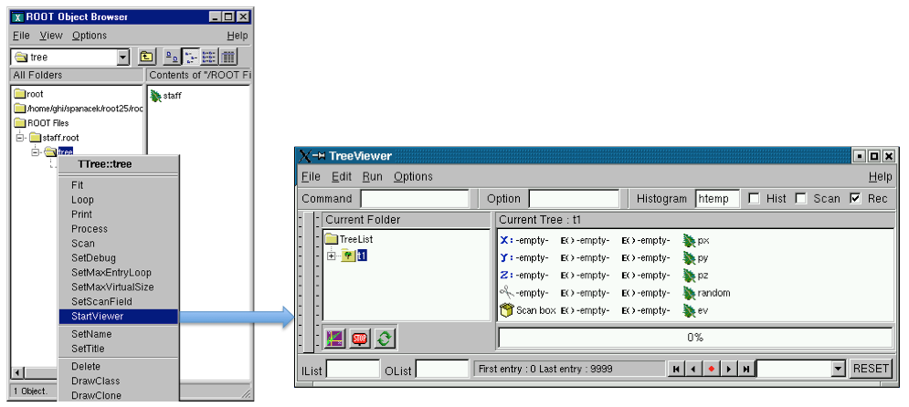
...The tree viewer is a quick and easy way to examine a tree. To start the tree viewer, open a file and object browser. Right click on a TTree and select StartViewer. You can also start the tree viewer from the command line. First load the viewer library.
If you want to start a tree viewer without a tree, you need to load the tree player library first:
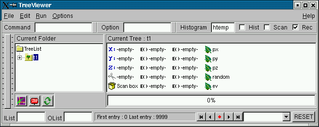
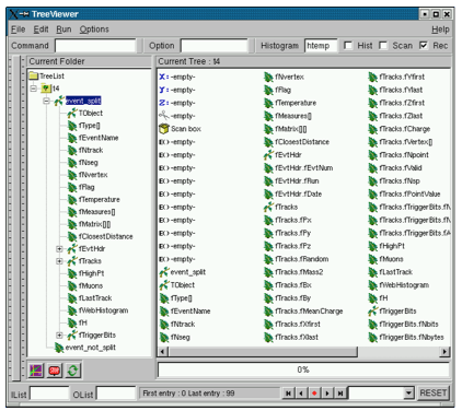
The figure above shows how the tree viewer looks like for the example file cernstaff.root. The left panel contains the list of trees and their branches; in this case there is only one tree. You can add more trees with the File-Open command to open the file containing the new tree, then use the context menu on the right panel, select SetTreeName and enter the name of the tree to add. On the right are the leaves or variables in the tree. You can double click on any leaf to a histogram it.
The toolbar in the upper part can be used for user commands, changing the drawing option and the histogram name. The lower part contains three picture buttons that draw a histogram, stop the current command, and refresh the tree.
The three check buttons toggle the following:
Hist- the histogram drawing mode;
Scan- enables redirecting of TTree::Scancommand in an ASCII file;
Rec - enables recording of the last issued command.
 To draw more than one dimension you can drag and drop any leaf to the
 X,Y,Z boxes". Then push the Draw button, witch is marked with the purple icon on the bottom left.
 All commands can be interrupted at any time by pressing this button.
 The method
 TTree::Refresh is called by pressing the refresh button in TTreeViewer. It redraws the current exposed expression. Calling TTree::Refresh is useful when a tree is produced by a writer process and concurrently analyzed by one or more readers.
 To add a cut/weight to the histogram, enter an expression in the “cut box”. The cut box is the one with the scissor icon.
Below them there are two text widgets for specifying the input and output event lists. A Tree Viewer session is made by the list of user-defined expressions and cuts, applying to a specified tree. A session can be saved using File / SaveSource menu or the SaveSource method from the context menu of the right panel. This will create a macro having as default name treeviewer.C that can be ran at any time to reproduce the session.
Besides the list of user-defined expressions, a session may contain a list of RECORDS. A record can be produced in the following way: dragging leaves/expression on X/Y/Z; changing drawing options; clicking the RED button on the bottom when happy with the histogram
NOTE that just double clicking a leaf will not produce a record: the histogram must be produced when clicking the DRAW button on the bottom-left. The records will appear on the list of records in the bottom right of the tree viewer. Selecting a record will draw the corresponding histogram. Records can be played using the arrow buttons near to the record button. When saving the session, the list of records is being saved as well.
Records have a default name corresponding to the Z: Y: X selection, but this can be changed using SetRecordName() method from the right panel context menu. You can create a new expression by right clicking on any of theE() boxes. The expression can be dragged and dropped into any of the boxes (X, Y, Z, Cut, or Scan). To scan one or more variables, drop them into the Scan box, then double click on the box. You can also redirect the result of the scan to a file by checking the Scan box on top.

When the “Rec” box is checked, the Draw and Scan commands are recorded in the history file and echoed on the command line. The “Histogram” text box contains the name of the resulting histogram. By default it is htemp. You can type any name, if the histogram does not exist it will create one. The Option text box contains the list of Draw options. See “Draw Options”. You can select the options with the Options menu. The Command box lets you enter any command that you could also enter on the command line. The vertical slider on the far left side can be used to select the minimum and maximum of an event range. The actual start and end index are shown in on the bottom in the status window.
There is an extensive help utility accessible with the Help menu. The IList and OList are to specify an input list of entry indices and a name for the output list respectively. Both need to be of type TList and contain integers of entry indices. These lists are described below in the paragraph “Error! Reference source not found.”.
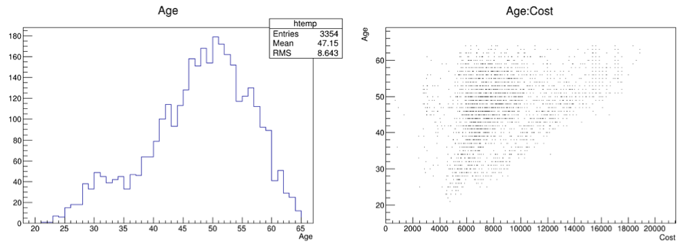
The first one is a plot of the age distribution, the second a scatter plot of the cost vs. age. The second one was generated by dragging the age leaf into the Y-box and the cost leaf into the X-box, and pressing the Draw button. By default, this will generate a scatter plot. Select a different option, for example "lego" to create a 2D histogram.
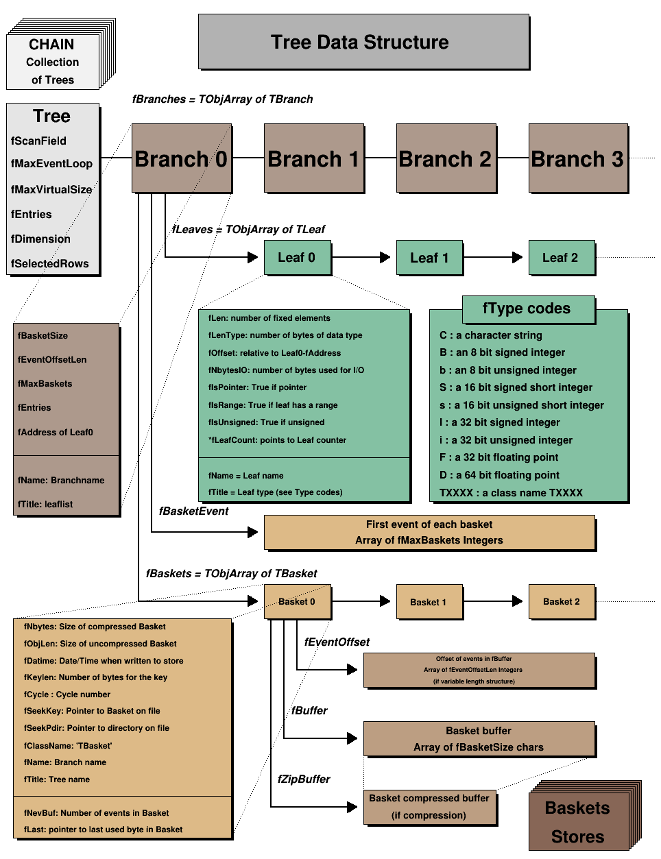
This picture shows the TTree class:
To create a TTree we use its constructor. Then we design our data layout and add the branches. A tree can be created by giving a name and title:
An alternative way to create a tree and organize it is to use folders (see “Folders and Tasks”). You can build a folder structure and create a tree with branches for each of the sub-folders:
The second argument "/MyFolder"is the top folder, and the “/” signals the TTree constructor that this is a folder not just the title. You fill the tree by placing the data into the folder structure and calling TTree::Fill.
This call requests the construction of an optional branch supporting table of references (TRefTable). This branch (TBranchRef) will keep all the information needed to find the branches containing referenced objects at each Tree::Fill, the branch numbers containing the referenced objects are saved in the table of references. When the Tree header is saved (via TTree::Write for example), the branch is saved, keeping the information with the pointers to the branches having referenced objects. Enabling this optional table, allow TTree::Draw to automatically load the branches needed to dereference a TRef (or TRefArray) object.
Autosave gives the option to save all branch buffers every n byte. We recommend using Autosave for large acquisitions. If the acquisition fails to complete, you can recover the file and all the contents since the last Autosave. To set the number of bytes between Autosave you can use the TTree::SetAutosave() method. You can also call TTree::Autosave in the acquisition loop every nentry.
When a TTree is memory resident, you set it up so that it retains retain only the last few entries. For example, this can be very useful for monitoring purpose.
where maxEntries is the maximum number of entries to be kept in the buffers. When the number of entries exceeds this value, the first entries in the Tree are deleted and the buffers used again. An example of a script using a circular buffer is shown below:
void circular() {
   gROOT->cd(); //make sure that the Tree is memory resident
   TTree *T = new TTree("T","test circular buffers");
   TRandom r;
   Float_t px,py,pz;
   Double_t random;
   UShort_t i;
   T->Branch("px",&px,"px/F");
   T->Branch("py",&py,"py/F");
   T->Branch("pz",&pz,"pz/F");
   T->Branch("random",&random,"random/D");
   T->Branch("i",&i,"i/s");
   T->SetCircular(20000);
   for (i = 0; i < 65000; i++) {
      r.Rannor(px,py);
      pz = px*px + py*py;
      random = r.Rndm();
      T->Fill();
   }
   T->Print();
}When writing a TTree to a file, if the file size reaches the value stored in the TTree::GetMaxTreeSize(), the current file is closed and a new file is created. If the original file is named “myfile.root”, subsequent files are named “myfile_1.root”, “myfile_2.root”, etc.
Currently, the automatic change of file is restricted to the case where the tree is in the top level directory. The file should not contain sub-directories. Before switching to a new file, the tree header is written to the current file, then the current file is closed. To process the multiple files created by ChangeFile(), one must use a TChain.
The new file name has a suffix “_N” where N is equal to fFileNumber+1. By default a Root session starts with fFileNumber=0. One can set fFileNumber to a different value via TTree::SetFileNumber(). In case a file named “_N” already exists, the function will try a file named “__N”, then “___N”, etc. The maximum tree size can be set via the static function TTree::SetMaxTreeSize(). The default value of fgMaxTreeSize is 100 GB. If the current file contains other objects (like TH1 and TTree), these objects are automatically moved to the new file.
The function TTree::GetUserInfo() allows adding any object defined by a user to the tree that is not depending on the entry number. For example:
Use TTree::BuildIndex(), to build an index table using expressions depending on the value in the leaves.
The index is built in the following way:
TTree::Draw()var1 = majornamevar2 = minornamesel = \(2^{31} \times majorname + minorname\)fIndexValuesOnce the index is computed, using the TTree::GetEntryWithIndex(majornumber, minornumber) one entry can be retrieved. Example:
   // to create an index using leaves Run and Event
   tree.BuildIndex("Run","Event");
   // to read entry corresponding to Run=1234 and Event=56789
   tree.GetEntryWithIndex(1234,56789);
Note that majorname and minorname may be expressions using original tree variables e.g.: “run-90000”, “event +3*xx”. In case an expression is specified, the equivalent expression must be computed when calling GetEntryWithIndex(). To build an index with only majorname, specify minorname="0" (default).
Note that once the index is built, it can be saved with the TTree object with:
The most convenient place to create the index is at the end of the filling process just before saving the tree header. If a previous index was computed, it is redefined by this new call.
Note that this function can also be applied to a TChain. The return value is the number of entries in the Index (< 0 indicates failure).
The organization of branches allows the designer to optimize the data for the anticipated use. The class for a branch is called TBranch. If two variables are independent, and the designer knows the variables will not be used together, they should be placed on separate branches. If, however, the variables are related, such as the coordinates of a point, it is most efficient to create one branch with both coordinates on it. A variable on a TBranch is called a leaf (yes - TLeaf). Another point to keep in mind when designing trees is that branches of the same TTree can be written to separate files. To add a TBranch to a TTree we call the method TTree::Branch(). Note that we DO NOT use the TBranch constructor.
The TTree::Branch method has several signatures. The branch type differs by what is stored in it. A branch can hold an entire object, a list of simple variables, contents of a folder, contents of a TList, or an array of objects. Let’s see some examples. To follow along you will need the shared library libEvent.so. First, check if it is in $ROOTSYS/test. If it is, copy it to your own area. If it is not there, you have to build it by typing make in $ROOTSYS/test.
As in the very first example (cernstaff.root.root) the data we want to save is a list of simple variables, such as integers or floats. In this case, we use the following TTree::Branch signature:
The first parameter is the branch name.
The second parameter is the address from which the first variable is to be read. In the code above, “event” is a structure with one float and three integers and one unsigned integer. You should not assume that the compiler aligns the elements of a structure without gaps. To avoid alignment problems, you need to use structures with same length members. If your structure does not qualify, you need to create one branch for each element of the structure.
The leaf name is NOT used to pick the variable out of the structure, but is only used as the name for the leaf. This means that the list of variables needs to be in a structure in the order described in the third parameter.
This third parameter is a string describing the leaf list. Each leaf has a name and a type separated by a “/” and it is separated from the next leaf by a “:”.
The example on the next line has two leafs: a floating-point number called temp and an integer named ntrack.
The type can be omitted and if no type is given, the same type as the previous variable is assumed. This leaf list has three integers called ntrack, nseg, and nvtex.
There is one more rule: when no type is given for the very first leaf, it becomes a float (F). This leaf list has three floats called temp, mass, and px.
The symbols used for the type are:
C: a character string terminated by the 0 characterB: an 8 bit signed integerb: an 8 bit unsigned integerS: a 16 bit signed integers: a 16 bit unsigned integerI: a 32 bit signed integeri: a 32 bit unsigned integerL: a 64 bit signed integerl: a 64 bit unsigned integerG: a long signed integer, stored as 64 bitg: a long unsigned integer, stored as 64 bitF: a 32 bit floating pointD: a 64 bit floating pointO: [the letter ‘o’, not a zero] a boolean (Bool_t)The type is used for a byte count to decide how much space to allocate. The variable written is simply the block of bytes starting at the starting address given in the second parameter. It may or may not match the leaf list depending on whether or not the programmer is being careful when choosing the leaf address, name, and type.
By default, a variable will be copied with the number of bytes specified in the type descriptor symbol. However, if the type consists of two characters, the number specifies the number of bytes to be used when copying the variable to the output buffer. The line below describes ntrack to be written as a 16-bit integer (rather than a 32-bit integer).
With this Branch method, you can also add a leaf that holds an entire array of variables. To add an array of floats use the f[n] notation when describing the leaf.
You can also add an array of variable length:
{
   TFile *f = new TFile("peter.root","recreate");
   Int_t nPhot;
   Float_t E[500];
   TTree* nEmcPhotons = new TTree("nEmcPhotons","EMC Photons");
   nEmcPhotons->Branch("nPhot",&nPhot,"nPhot/I");
   nEmcPhotons->Branch("E",E,"E[nPhot]/F");
}
See “Example 2: A Tree with a C Structure” below ($ROOTSYS/tutorials/tree/tree2.C) and staff.C at the beginning of this chapter.
To write a branch to hold an event object, we need to load the definition of the Event class, which is in $ROOTSYS/test/libEvent.so (if it doesn’t exist type make in $ROOTSYS/test). An object can be saved in a tree if a ROOT dictionary for its class has been generated and loaded.
First, we need to open a file and create a tree.
root[]     TFile *f = new TFile("AFile.root","RECREATE")
root[]     TTree *tree = new TTree("T","A Root Tree")
We need to create a pointer to an Event object that will be used as a reference in the TTree::Branch method. Then we create a branch with the TTree::Branch method.
To add a branch to hold an object we use the signature above. The first parameter is the name of the branch. The second parameter is the name of the class of the object to be stored. The third parameter is the address of a pointer to the object to be stored.
Note that it is an address of a pointer to the object, not just a pointer to the object.
The fourth parameter is the buffer size and is by default 32000 bytes. It is the number of bytes of data for that branch to save to a buffer until it is saved to the file. The last parameter is the split-level, which is the topic of the next section. Static class members are not part of an object and thus not written with the object. You could store them separately by collecting these values in a special “status” object and write it to the file outside of the tree. If it makes sense to store them for each object, make them a regular data member.
To split a branch means to create a sub-branch for each data member in the object. The split-level can be set to 0 to disable splitting or it can be set to a number between 1 and 99 indicating the depth of splitting.
If the split-level is set to zero, the whole object is written in its entirety to one branch. The TTree will look like the one on the right, with one branch and one leaf holding the entire event object.
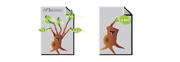
When the split-level is 1, an object data member is assigned a branch. If the split-level is 2, the data member objects will be split also, and a split level of 3 its data members objects, will be split. As the split-level increases so does the splitting depth. The ROOT default for the split-level is 99. This means the object will be split to the maximum.
Splitting a branch can quickly generate many branches. Each branch has its own buffer in memory. In case of many branches (say more than 100), you should adjust the buffer size accordingly. A recommended buffer size is 32000 bytes if you have less than 50 branches. Around 16000 bytes if you have less than 100 branches and 4000 bytes if you have more than 500 branches. These numbers are recommended for computers with memory size ranging from 32MB to 256MB. If you have more memory, you should specify larger buffer sizes. However, in this case, do not forget that your file might be used on another machine with a smaller memory configuration.
A split branch is faster to read, but slightly slower to write. The reading is quicker because variables of the same type are stored consecutively and the type does not have to be read each time. It is slower to write because of the large number of buffers as described above. See "
Performance Benchmarks" for performance impact of split and non-split mode.
When splitting a branch, variables of different types are handled differently. Here are the rules that apply when splitting a branch.
If a data member is a basic type, it becomes one branch of class TBranchElement.
A data member can be an array of basic types. In this case, one single branch is created for the array.
A data member can be a pointer to an array of basic types. The length can vary, and must be specified in the comment field of the data member in the class definition. See “Input/Output”.
Pointer data member are not split, except for pointers to a TClonesArray. The TClonesArray (pointed to) is split if the split level is greater than two. When the split level is one, the TClonesArray is not split.
If a data member is a pointer to an object, a special branch is created. The branch will be filled by calling the class Streamer function to serialize the object into the branch buffer.
If a data member is an object, the data members of this object are split into branches according to the split-level (i.e. split-level > 2).
Base classes are split when the object is split.
Abstract base classes are never split.
All STL containers are supported.
   // STL vector of vectors of TAxis*
   vector<vector<TAxis *> >  fVectAxis;
   // STL map of string/vector
   map<string,vector<int> >  fMapString;
   // STL deque of pair
   deque<pair<float,float> > fDequePair;
C-structure data members are not supported in split mode.
An object that is not split may be slow to browse.
A STL container that is not split will not be accessible in the browser.
If you are creating a branch with an object and in general you want the data members to be split, but you want to exempt a data member from the split. You can specify this in the comment field of the data member:
ROOT has two classes to manage arrays of objects. The TObjArray can manage objects of different classes, and the TClonesArray that specializes in managing objects of the same class (hence the name Clones Array). TClonesArray takes advantage of the constant size of each element when adding the elements to the array. Instead of allocating memory for each new object as it is added, it reuses the memory. Here is an example of the time a TClonesArray can save over a TObjArray. We have 100,000 events, and each has 10,000 tracks, which gives 1,000,000,000 tracks. If we use a TObjArray for the tracks, we implicitly make a call to new and a corresponding call to delete for each track. The time it takes to make a pair of new/delete calls is about 7 s (10-6). If we multiply the number of tracks by 7 s, (1,000,000,000 * 7 * 10-6) we calculate that the time allocating and freeing memory is about 2 hours. This is the chunk of time saved when a TClonesArray is used rather than a TObjArray. If you do not want to wait 2 hours for your tracks (or equivalent objects), be sure to use a TClonesArray for same-class objects arrays. Branches with TClonesArrays use the same method (TTree::Branch) as any other object described above. If splitting is specified the objects in the TClonesArray are split, not the TClonesArray itself.
When a top-level object (say event), has two data members of the same class the sub branches end up with identical names. To distinguish the sub branch we must associate them with the master branch by including a “.” (a dot) at the end of the master branch name. This will force the name of the sub branch to be master.sub branch instead of simply sub branch. For example, a tree has two branches Trigger and MuonTrigger, each containing an object of the same class (Trigger). To identify uniquely the sub branches we add the dot:
If Trigger has three members, T1, T2, T3, the two instructions above will generate sub branches called: Trigger.T1, Trigger.T2, Trigger.T3, MuonTrigger.T1, MuonTrigger.T2, andMuonTrigger.T3.
Use the syntax below to add a branch from a folder:
This method creates one branch for each element in the folder. The method returns the total number of branches created.
This Branch method creates one branch for each element in the collection.
   tree->Branch(*aCollection, 8000, 99);
   // Int_t TTree::Branch(TCollection *list, Int_t bufsize,
   //                     Int_t splitlevel, const char *name)
The method returns the total number of branches created. Each entry in the collection becomes a top level branch if the corresponding class is not a collection. If it is a collection, the entry in the collection becomes in turn top level branches, etc. The split level is decreased by 1 every time a new collection is found. For example if list is a TObjArray*
If splitlevel = 1, one top level branch is created for each element of the TObjArray.
If splitlevel = 2, one top level branch is created for each array element. If one of the array elements is a TCollection, one top level branch will be created for each element of this collection.
In case a collection element is a TClonesArray, the special Tree constructor for TClonesArray is called. The collection itself cannot be a TClonesArray. If name is given, all branch names will be prefixed with name_.
IMPORTANT NOTE1: This function should not be called if splitlevel<1. IMPORTANT NOTE2: The branches created by this function will have names corresponding to the collection or object names. It is important to give names to collections to avoid misleading branch names or identical branch names. By default collections have a name equal to the corresponding class name, e.g. the default name of TList is “TList”.
The following sections are examples of writing and reading trees increasing in complexity from a simple tree with a few variables to a tree containing folders and complex Event objects. Each example has a named script in the $ROOTSYS/tutorials/tree directory. They are called tree1.C to tree4.C. The examples are:
tree1.C: a tree with several simple (integers and floating point) variables.
tree2.C: a tree built from a C structure (struct). This example uses the Geant3 C wrapper as an example of a FORTRAN common block ported to C with a C structure.
tree3.C: in this example, we will show how to extend a tree with a branch from another tree with the Friends feature. These trees have branches with variable length arrays. Each entry has a variable number of tracks, and each track has several variables.
tree4.C: a tree with a class (Event). The class Event is defined in $ROOTSYS/test. In this example we first encounter the impact of splitting a branch.
Each script contains the main function, with the same name as the file (i.e. tree1), the function to write - tree1w, and the function to read - tree1r. If the script is not run in batch mode, it displays the tree in the browser and tree viewer. To study the example scripts, you can either execute the main script, or load the script and execute a specific function. For example:
// execute the function that writes, reads, shows the tree
root[]     x tree1.C
// use ACLiC to build shared library, check syntax, execute
root[] x tree1.C++
// Load the script and select a function to execute
root[]     L tree1.C
root[]     tree1w()
root[] tree1r()This example shows how to write, view, and read a tree with several simple (integers and floating-point) variables.
Below is the function that writes the tree (tree1w). First, the variables are defined (px, py, pz, random and ev). Then we add a branch for each of the variables to the tree, by calling the TTree::Branch method for each variable.
void tree1w(){

   // create a tree file tree1.root - create the file, the Tree and
   // a few branches
   TFile f("tree1.root","recreate");
   TTree t1("t1","a simple Tree with simple variables");
   Float_t px, py, pz;
   Double_t random;
   Int_t ev;
   t1.Branch("px",&px,"px/F");
   t1.Branch("py",&py,"py/F");
   t1.Branch("pz",&pz,"pz/F");
   t1.Branch("ev",&ev,"ev/I");

   // fill the tree
   for (Int_t i=0; i<10000; i++) {
      gRandom->Rannor(px,py);
      pz = px*px + py*py;
      random = gRandom->Rndm();
      ev = i;
      t1.Fill();
   }
   // save the Tree heade; the file will be automatically closed
   // when going out of the function scope
   t1.Write();
}This is the signature of TTree::Branch to create a branch with a list of variables:
The first parameter is the branch name. The second parameter is the address from which to read the value. The third parameter is the leaf list with the name and type of each leaf. In this example, each branch has only one leaf. In the box below, the branch is named px and has one floating point type leaf also called px.
First we find some random values for the variables. We assign px and py a Gaussian with mean = 0 and sigma = 1 by calling gRandom->Rannor(px,py), and calculatepz. Then we call the TTree::Fill() method. The call t1.Fill() fills all branches in the tree because we have already organized the tree into branches and told each branch where to get the value from. After this script is executed we have a ROOT file called tree1.root with a tree called t1. There is a possibility to fill branches one by one using the method TBranch::Fill(). In this case you do not need to call TTree::Fill() method. The entries can be set by TTree::SetEntries(Double_t n). Calling this method makes sense only if the number of existing entries is null.
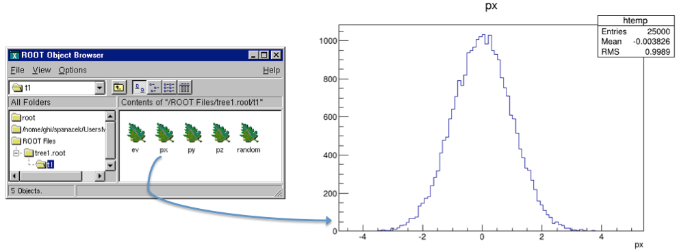
In the right panel of the ROOT object browse are the branches: ev, px, py, pz, and random. Note that these are shown as leaves because they are “end” branches with only one leaf. To histogram a leaf, we can simply double click on it in the browser. This is how the tree t1 looks in the Tree Viewer. Here we can add a cut and add other operations for histogramming the leaves. See “The Tree Viewer”. For example, we can plot a two dimensional histogram.
The tree1r function shows how to read the tree and access each entry and each leaf. We first define the variables to hold the read values.
Then we tell the tree to populate these variables when reading an entry. We do this with the method TTree::SetBranchAddress. The first parameter is the branch name, and the second is the address of the variable where the branch data is to be placed. In this example, the branch name is px. This name was given when the tree was written (see tree1w). The second parameter is the address of the variable px.
Once the branches have been given the address, a specific entry can be read into the variables with the method TTree::GetEntry(n). It reads all the branches for entry (n) and populates the given address accordingly. By default, GetEntry() reuses the space allocated by the previous object for each branch. You can force the previous object to be automatically deleted if you call mybranch.SetAutoDelete(kTRUE) (default is kFALSE).
Consider the example in $ROOTSYS/test/Event.h. The top-level branch in the tree T is declared with:
   Event *event = 0;
   // event must be null or point to a valid object;
   // it must be initialized
   T.SetBranchAddress("event",&event);
When reading the Tree, one can choose one of these 3 options:
Option 1:
   for (Int_t i = 0; i<nentries; i++) {
      T.GetEntry(i);
      //the object event has been filled at this point
   }
This is the default and recommended way to create an object of the class Event.It will be pointed by event.
At the following entries, event will be overwritten by the new data. All internal members that are TObject* are automatically deleted. It is important that these members be in a valid state when GetEntry is called. Pointers must be correctly initialized. However these internal members will not be deleted if the characters “->” are specified as the first characters in the comment field of the data member declaration.
The pointer member is read via the pointer->Streamer(buf) if “->” is specified. In this case, it is assumed that the pointer is never null (see pointer TClonesArray *fTracks in the $ROOTSYS/test/Event example). If “->” is not specified, the pointer member is read via buf >> pointer. In this case the pointer may be null. Note that the option with “->” is faster to read or write and it also consumes less space in the file.
Option 2 - the option AutoDelete is set:
   TBranch *branch = T.GetBranch("event");
   branch->SetAddress(&event);
   branch->SetAutoDelete(kTRUE);
   for (Int_t i=0; i<nentries; i++) {
      T.GetEntry(i); // the object event has been filled at this point
   }
At any iteration, the GetEntry deletes the object event and a new instance of Event is created and filled.
Option 3 - same as option 1, but you delete the event yourself:
   for (Int_t i=0; i<nentries; i++) {
      delete event;
      event = 0;      //EXTREMELY IMPORTANT
      T.GetEntry(i);
      // the objrect event has been filled at this point
   }
It is strongly recommended to use the default option 1. It has the additional advantage that functions like TTree::Draw (internally calling TTree::GetEntry) will be functional even when the classes in the file are not available. Reading selected branches is quicker than reading an entire entry. If you are interested in only one branch, you can use the TBranch::GetEntry method and only that branch is read. Here is the script tree1r:
void tree1r(){
   // read the Tree generated by tree1w and fill two histograms
   // note that we use "new" to create the TFile and TTree objects,
   // to keep them alive after leaving this function.
   TFile *f = new TFile("tree1.root");
   TTree *t1 = (TTree*)f->Get("t1");
   Float_t px, py, pz;
   Double_t random;
   Int_t ev;
   t1->SetBranchAddress("px",&px);
   t1->SetBranchAddress("py",&py);
   t1->SetBranchAddress("pz",&pz);
   t1->SetBranchAddress("random",&random);
   t1->SetBranchAddress("ev",&ev);
   // create two histograms
   TH1F *hpx   = new TH1F("hpx","px distribution",100,-3,3);
   TH2F *hpxpy = new TH2F("hpxpy","py vs px",30,-3,3,30,-3,3);
   //read all entries and fill the histograms
   Int_t nentries = (Int_t)t1->GetEntries();
   for (Int_t i=0; i<nentries; i++) {
      t1->GetEntry(i);
      hpx->Fill(px);
      hpxpy->Fill(px,py);
   }
   // We do not close the file. We want to keep the generated
   // histograms we open a browser and the TreeViewer
   if (gROOT->IsBatch()) return;
   new TBrowser ();
   t1->StartViewer();

   //In the browser, click on "ROOT Files", then on "tree1.root"
   //You can click on the histogram icons in the right panel to draw
   //them in the TreeViewer, follow the instructions in the Help.
}The executable script for this example is $ROOTSYS/tutorials/tree/tree2.C.In this example we show:
TTree::Draw to show a 3D plotA C structure (struct) is used to build a ROOT tree. In general we discourage the use of C structures, we recommend using a class instead. However, we do support them for legacy applications written in C or FORTRAN. The example struct holds simple variables and arrays. It maps to a Geant3 common block /gctrak/.This is the definition of the common block/structure:
const Int_t MAXMEC = 30;
// PARAMETER (MAXMEC=30)
// COMMON/GCTRAK/VECT(7),GETOT,GEKIN,VOUT(7)
//     + ,NMEC,LMEC(MAXMEC)
//     + ,NAMEC(MAXMEC),NSTEP
//     + ,PID,DESTEP,DESTEL,SAFETY,SLENG
//     + ,STEP,SNEXT,SFIELD,TOFG,GEKRAT,UPWGHT

typedef struct {
   Float_t  vect[7];
   Float_t  getot;
   Float_t  gekin;
   Float_t  vout[7];
   Int_t    nmec;
   Int_t    lmec[MAXMEC];
   Int_t    namec[MAXMEC];
   Int_t    nstep;
   Int_t    pid;
   Float_t  destep;
   Float_t  destel;
   Float_t  safety;
   Float_t  sleng;
   Float_t  step;
   Float_t  snext;
   Float_t  sfield;
   Float_t  tofg;
   Float_t  gekrat;
   Float_t  upwght;
} Gctrak_t;
When using Geant3, the common block is filled by Geant3 routines at each step and only the TTree::Fill method needs to be called. In this example we emulate the Geant3 step routine with the helixStep function. We also emulate the filling of the particle values. The calls to the Branch methods are the same as if Geant3 were used.
void helixStep(Float_t step, Float_t *vect, Float_t *vout)
{
   // extrapolate track in constant field
   Float_t field = 20; // field in kilogauss
   enum Evect {kX,kY,kZ,kPX,kPY,kPZ,kPP};
   vout[kPP] = vect[kPP];

   Float_t h4    = field*2.99792e-4;
   Float_t rho   = -h4/vect[kPP];
   Float_t tet   = rho*step;
   Float_t tsint = tet*tet/6;
   Float_t sintt = 1 - tsint;
   Float_t sint  = tet*sintt;
   Float_t cos1t = tet/2;
   Float_t f1 = step*sintt;
   Float_t f2 = step*cos1t;
   Float_t f3 = step*tsint*vect[kPZ];
   Float_t f4 = -tet*cos1t;
   Float_t f5 = sint;
   Float_t f6 = tet*cos1t*vect[kPZ];

   vout[kX]  = vect[kX]  + (f1*vect[kPX] - f2*vect[kPY]);
   vout[kY]  = vect[kY]  + (f1*vect[kPY] + f2*vect[kPX]);
   vout[kZ]  = vect[kZ]  + (f1*vect[kPZ] + f3);
   vout[kPX] = vect[kPX] + (f4*vect[kPX] - f5*vect[kPY]);
   vout[kPY] = vect[kPY] + (f4*vect[kPY] + f5*vect[kPX]);
   vout[kPZ] = vect[kPZ] + (f4*vect[kPZ] + f6);
}void tree2w() {
// write tree2 example
//create a Tree file tree2.root
TFile f("tree2.root","recreate");
//create the file, the Tree
TTree t2("t2","a Tree with data from a fake Geant3");
// declare a variable of the C structure type
Gctrak_t gstep;
// add the branches for a subset of gstep
   t2.Branch("vect",gstep.vect,"vect[7]/F");
   t2.Branch("getot",&gstep.getot,"getot/F");
   t2.Branch("gekin",&gstep.gekin,"gekin/F");
   t2.Branch("nmec",&gstep.nmec,"nmec/I");
   t2.Branch("lmec",gstep.lmec,"lmec[nmec]/I");
t2.Branch("destep",&gstep.destep,"destep/F");
t2.Branch("pid",&gstep.pid,"pid/I");
//Initialize particle parameters at first point
Float_t px,py,pz,p,charge=0;
Float_t vout[7];
Float_t mass = 0.137;
Bool_t newParticle = kTRUE;
gstep.step = 0.1;
gstep.destep = 0;
gstep.nmec = 0;
gstep.pid = 0;
//transport particles
for (Int_t i=0; i<10000; i++) {
//generate a new particle if necessary (Geant3 emulation)
if (newParticle) {
px = gRandom->Gaus(0,.02);
py = gRandom->Gaus(0,.02);
pz = gRandom->Gaus(0,.02);
p = TMath::Sqrt(px*px+py*py+pz*pz);
charge = 1;
if (gRandom->Rndm() < 0.5) charge = -1;
gstep.pid += 1;
gstep.vect[0] = 0;
gstep.vect[1] = 0;
gstep.vect[2] = 0;
gstep.vect[3] = px/p;
gstep.vect[4] = py/p;
gstep.vect[5] = pz/p;
gstep.vect[6] = p*charge;
gstep.getot = TMath::Sqrt(p*p + mass*mass);
gstep.gekin = gstep.getot - mass;
newParticle = kFALSE;
}
// fill the Tree with current step parameters
t2.Fill();
//transport particle in magnetic field (Geant3 emulation)
helixStep(gstep.step, gstep.vect, vout);
//make one step
//apply energy loss
gstep.destep = gstep.step*gRandom->Gaus(0.0002,0.00001);
gstep.gekin -= gstep.destep;
gstep.getot = gstep.gekin + mass;
gstep.vect[6]= charge*TMath::Sqrt(gstep.getot*gstep.getot
- mass*mass);
gstep.vect[0] = vout[0];
gstep.vect[1] = vout[1];
gstep.vect[2] = vout[2];
gstep.vect[3] = vout[3];
gstep.vect[4] = vout[4];
gstep.vect[5] = vout[5];
gstep.nmec = (Int_t)(5*gRandom->Rndm());
for (Int_t l=0; l<gstep.nmec; l++) gstep.lmec[l] = l;
if (gstep.gekin < 0.001) newParticle = kTRUE;
if (TMath::Abs(gstep.vect[2]) > 30) newParticle = kTRUE;
}
//save the Tree header. The file will be automatically
// closed when going out of the function scope
t2.Write();
}At first, we create a tree and create branches for a subset of variables in the C structureGctrak_t. Then we add several types of branches. The first branch reads seven floating-point values beginning at the address of 'gstep.vect'. You do not need to specify &gstep.vect, because in C and C++ the array variable holds the address of the first element.
t2.Branch("vect",gstep.vect,"vect[7]/F");
t2.Branch("getot",&gstep.getot,"getot/F");
t2.Branch("gekin",&gstep.gekin,"gekin/F");The next two branches are dependent on each other. The first holds the length of the variable length array and the second holds the variable length array. The lmec branch reads nmec number of integers beginning at the address gstep.lmec.
The variable nmec is a random number and is reset for each entry.
In this emulation of Geant3, we generate and transport particles in a magnetic field and store the particle parameters at each tracking step in a ROOT tree.
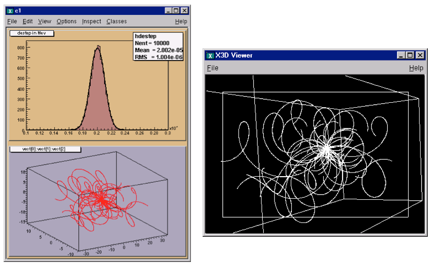
In this analysis, we do not read the entire entry we only read one branch. First, we set the address for the branch to the file dstep, and then we use the TBranch::GetEntry method. Then we fill a histogram with the dstep branch entries, draw it and fit it with a Gaussian. In addition, we draw the particle’s path using the three values in the vector. Here we use the TTree::Draw method. It automatically creates a histogram and plots the 3 expressions (see Trees in Analysis).
void tree2r() {

   // read the Tree generated by tree2w and fill one histogram
   // we are only interested by the destep branch

   // note that we use "new" to create the TFile and TTree objects because we
   // want to keep these objects alive when we leave this function
   TFile *f = new TFile("tree2.root");
   TTree *t2 = (TTree*)f->Get("t2");
   static Float_t destep;
   TBranch *b_destep = t2->GetBranch("destep");
   b_destep->SetAddress(&destep);

   //create one histogram
   TH1F *hdestep = new TH1F("hdestep","destep in Mev",100,1e-5,3e-5);
   //read only the destep branch for all entries
   Int_t nentries = (Int_t)t2->GetEntries();
   for (Int_t i=0;i<nentries;i++) {
      b_destep->GetEntry(i);
      // fill the histogram with the destep entry
      hdestep->Fill(destep);
   }

   // we do not close the file; we want to keep the generated histograms;
   // we fill a 3-d scatter plot with the particle step coordinates
   TCanvas *c1 = new TCanvas("c1","c1",600,800);
   c1->SetFillColor(42);
   c1->Divide(1,2);

   c1->cd(1);
   hdestep->SetFillColor(45);
   hdestep->Fit("gaus");

   c1->cd(2);
   gPad->SetFillColor(37);                       // continued...
   t2->SetMarkerColor(kRed);
   t2->Draw("vect[0]:vect[1]:vect[2]");
   if (gROOT->IsBatch()) return;

   // invoke the x3d viewer
   gPad->GetViewer3D("x3d");
}In this example, we will show how to extend a tree with a branch from another tree with the Friends feature.
You may want to add a branch to an existing tree. For example, if one variable in the tree was computed with a certain algorithm, you may want to try another algorithm and compare the results. One solution is to add a new branch, fill it, and save the tree. The code below adds a simple branch to an existing tree. Note that the kOverwrite option in the Write method overwrites the existing tree. If it is not specified, two copies of the tree headers are saved.
void tree3AddBranch() {
   TFile f("tree3.root","update");
   Float_t new_v;
   TTree *t3 = (TTree*)f->Get("t3");
   TBranch *newBranch = t3-> Branch("new_v",&new_v,"new_v/F");
   //read the number of entries in the t3
   Int_t nentries = (Int_t)t3->GetEntries();
   for (Int_t i = 0; i < nentries; i++){
      new_v= gRandom->Gaus(0,1);
      newBranch->Fill();
   }
   t3->Write("",TObject::kOverwrite); // save only the new version of
                                      // the tree
}
Adding a branch is often not possible because the tree is in a read-only file and you do not have permission to save the modified tree with the new branch. Even if you do have the permission, you risk loosing the original tree with an unsuccessful attempt to save the modification. Since trees are usually large, adding a branch could extend it over the 2GB limit. In this case, the attempt to write the tree fails, and the original data is may also be corrupted. In addition, adding a branch to a tree enlarges the tree and increases the amount of memory needed to read an entry, and therefore decreases the performance. For these reasons, ROOT offers the concept of friends for trees (and chains). We encourage you to use TTree::AddFriend rather than adding a branch manually.
A tree keeps a list of friends. In the context of a tree (or a chain), friendship means unrestricted access to the friends data. In this way it is much like adding another branch to the tree without taking the risk of damaging it. To add a friend to the list, you can use the TTree::AddFriend method. The TTree (tree) below has two friends (ft1 and ft2) and now has access to the variables a,b,c,i,j,k,l and m.
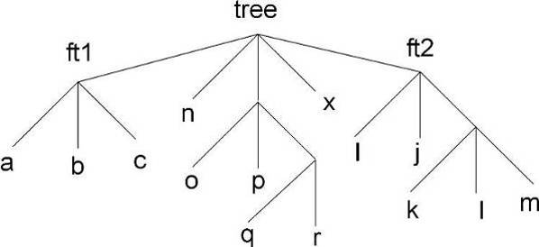
The AddFriend method has two parameters, the first is the tree name and the second is the name of the ROOT file where the friend tree is saved. AddFriend automatically opens the friend file. If no file name is given, the tree called ft1 is assumed to be in the same file as the original tree.
If the friend tree has the same name as the original tree, you can give it an alias in the context of the friendship:
Once the tree has friends, we can use TTree::Draw as if the friend’s variables were in the original tree. To specify which tree to use in the Draw method, use the syntax:
If the variablename is enough to identify uniquely the variable, you can leave out the tree and/or branch name.
For example, these commands generate a 3-d scatter plot of variable “var” in the TTree tree versus variable v1 inTTree ft1versus variablev2in **TTree**ft2`.
tree.AddFriend("ft1","friendfile1.root");
tree.AddFriend("ft2","friendfile2.root");
tree.Draw("var:ft1.v1:ft2.v2");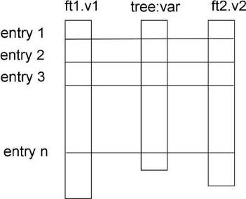 The picture illustrates the access of the tree and its friends with a
 Draw command.
When AddFriend is called, the ROOT file is automatically opened and the friend tree (ft1) header is read into memory. The new friend (ft1) is added to the list of friends of tree. The number of entries in the friend must be equal or greater to the number of entries of the original tree. If the friend tree has fewer entries, a warning is given and the missing entries are not included in the histogram.
Use TTree::GetListOfFriends to retrieve the list of friends from a tree.
When the tree is written to file (TTree::Write), the friends list is saved with it. Moreover, when the tree is retrieved, the trees on the friends list are also retrieved and the friendship restored. When a tree is deleted, the elements of the friend list are also deleted. It is possible to declare a friend tree that has the same internal structure (same branches and leaves) as the original tree, and compare the same values by specifying the tree.
The example code is in $ROOTSYS/tutorials/tree/tree3.C. Here is the script:
void tree3w() {
   // Example of a Tree where branches are variable length arrays
   // A second Tree is created and filled in parallel.
   // Run this script with .x tree3.C
   // In the function treer, the first Tree is open.
   // The second Tree is declared friend of the first tree.
   // TTree::Draw is called with variables from both Trees.
   const Int_t kMaxTrack = 500;
   Int_t ntrack;
   Int_t stat[kMaxTrack];
   Int_t sign[kMaxTrack];
   Float_t px[kMaxTrack];
   Float_t py[kMaxTrack];
   Float_t pz[kMaxTrack];
   Float_t pt[kMaxTrack];
   Float_t zv[kMaxTrack];
   Float_t chi2[kMaxTrack];
   Double_t sumstat;

   // create the first root file with a tree
   TFile f("tree3.root","recreate");
   TTree *t3 = new TTree("t3","Reconst ntuple");
   t3->Branch("ntrack",&ntrack,"ntrack/I");
   t3->Branch("stat",stat,"stat[ntrack]/I");
   t3->Branch("sign",sign,"sign[ntrack]/I");
   t3->Branch("px",px,"px[ntrack]/F");
   t3->Branch("py",py,"py[ntrack]/F");
   t3->Branch("pz",pz,"pz[ntrack]/F");
   t3->Branch("zv",zv,"zv[ntrack]/F");
   t3->Branch("chi2",chi2,"chi2[ntrack]/F");

   // create the second root file with a different tree
   TFile fr("tree3f.root","recreate");
   TTree *t3f = new TTree("t3f","a friend Tree");
   t3f->Branch("ntrack",&ntrack,"ntrack/I");
   t3f->Branch("sumstat",&sumstat,"sumstat/D");
   t3f->Branch("pt",pt,"pt[ntrack]/F");

   // Fill the trees
   for (Int_t i=0;i<1000;i++) {
      Int_t nt = gRandom->Rndm()*(kMaxTrack-1);
      ntrack = nt;
      sumstat = 0;
      // set the values in each track
      for (Int_t n=0;n<nt;n++) {
         stat[n] = n%3;
         sign[n] = i%2;
         px[n]   = gRandom->Gaus(0,1);
         py[n]   = gRandom->Gaus(0,2);
         pz[n]   = gRandom->Gaus(10,5);
         zv[n]   = gRandom->Gaus(100,2);
         chi2[n] = gRandom->Gaus(0,.01);
         sumstat += chi2[n];
         pt[n]   = TMath::Sqrt(px[n]*px[n] + py[n]*py[n]);
      }
      t3->Fill();
      t3f->Fill();
   }
   // Write the two files
   t3->Print();
   f.cd();
   t3->Write();
   fr.cd();
   t3f->Write();
}

// Function to read the two files and add the friend
void tree3r()         {
   TFile *f = new TFile("tree3.root");
   TTree *t3 = (TTree*)f->Get("t3");
   // Add the second tree to the first tree as a friend
   t3->AddFriend("t3f","tree3f.root");
   // Draw pz which is in the first tree and use pt
   // in the condition. pt is in the friend tree.
   t3->Draw("pz","pt>3");
}

// This is executed when typing .x tree3.C
void tree3() {
   tree3w();
   tree3r();
}This example is a simplified version of $ROOTSYS/test/MainEvent.cxx and where Event objects are saved in a tree. The full definition of Event is in $ROOTSYS/test/Event.h. To execute this macro, you will need the library $ROOTSYS/test/libEvent.so. If it does not exist you can build the test directory applications by following the instruction in the $ROOTSYS/test/README file.
In this example we will show
Event is a descendent of TObject. As such it inherits the data members of TObject and its methods such as Dump() and Inspect()andWrite(). In addition, because it inherits from TObject it can be a member of a collection. To summarize, the advantages of inheriting from a TObject are:
Write, Inspect, and Dump methodsBelow is the list of the Event data members. It contains a character array, several integers, a floating-point number, and an EventHeader object. The EventHeader class is described in the following paragraph. Event also has two pointers, one to a TClonesArray of tracks and one to a histogram. The string “->” in the comment field of the members *fTracks and *fH instructs the automatic Streamer to assume that the objects *fTracks and *fH are never null pointers and that fTracks->Streamer can be used instead of the more time consuming form R__b << fTracks.
class Event : public TObject {
   private:
      char                 fType[20];
      Int_t                fNtrack;
      Int_t                fNseg;
      Int_t                fNvertex;
      UInt_t               fFlag;
      Float_t              fTemperature;
      EventHeader          fEvtHdr;
      TClonesArray        *fTracks;            //->
      TH1F                *fH;                 //->
      Int_t                fMeasures[10];
      Float_t              fMatrix[4][4];
      Float_t             *fClosestDistance;   //[fNvertex]
      static TClonesArray *fgTracks;
      static TH1F         *fgHist;
      // ... list of methods
      ClassDef(Event,1)  //Event structure
};The EventHeader class (also defined in Event.h) does not inherit from TObject. Beginning with ROOT 3.0, an object can be placed on a branch even though it does not inherit from TObject. In previous releases branches were restricted to objects inheriting from the TObject. However, it has always been possible to write a class not inheriting from TObject to a tree by encapsulating it in a TObject descending class as is the case in EventHeader and Event.
class EventHeader {
   private:
      Int_t   fEvtNum;
      Int_t   fRun;
      Int_t   fDate;
      // ... list of methods
      ClassDef(EventHeader,1)      //Event Header
};The Track class descends from TObject since tracks are in a TClonesArray (i.e. a ROOT collection class) and contains a selection of basic types and an array of vertices. Its TObject inheritance enables Track to be in a collection and in Event is a TClonesArray of Tracks.
class Track : public TObject {
   private:
      Float_t   fPx;         //X component of the momentum
      Float_t   fPy;         //Y component of the momentum
      Float_t   fPz;         //Z component of the momentum
      Float_t   fRandom;     //A random track quantity
      Float_t   fMass2;      //The mass square of this particle
      Float_t   fBx;         //X intercept at the vertex
      Float_t   fBy;         //Y intercept at the vertex
      Float_t   fMeanCharge; //Mean charge deposition of all hits
      Float_t   fXfirst;     //X coordinate of the first point
      Float_t   fXlast;      //X coordinate of the last point
      Float_t   fYfirst;     //Y coordinate of the first point
      Float_t   fYlast;      //Y coordinate of the last point
      Float_t   fZfirst;     //Z coordinate of the first point
      Float_t   fZlast;      //Z coordinate of the last point
      Float_t   fCharge;     //Charge of this track
      Float_t   fVertex[3];  //Track vertex position
      Int_t     fNpoint;     //Number of points for this track
      Short_t   fValid;      //Validity criterion

      // method definitions ...
      ClassDef(Track,1)          //A track segment
};We create a simple tree with two branches both holding Event objects. One is split and the other is not. We also create a pointer to an Event object (event).
void tree4w() {
   // check to see if the event class is in the dictionary
   // if it is not load the definition in libEvent.so
   if (!TClassTable::GetDict("Event")) {
      gSystem->Load("$ROOTSYS/test/libEvent.so");
   }
   // create a Tree file tree4.root
   TFile f("tree4.root","RECREATE");
   // create a ROOT Tree
   TTree t4("t4","A Tree with Events");
   // create a pointer to an Event object
   Event *event = new Event();
   // create two branches, split one
   t4.Branch("event_branch", "Event", &event,16000,2);
   t4.Branch("event_not_split", "Event", &event,16000,0);

   // a local variable for the event type
   char etype[20];

   // fill the tree
   for (Int_t ev = 0; ev <100; ev++) {
      Float_t sigmat, sigmas;
      gRandom->Rannor(sigmat,sigmas);
      Int_t ntrack   = Int_t(600 + 600 *sigmat/120.);
      Float_t random = gRandom->Rndm(1);
      sprintf(etype,"type%d",ev%5);
      event->SetType(etype);
      event->SetHeader(ev, 200, 960312, random);
      event->SetNseg(Int_t(10*ntrack+20*sigmas));
      event->SetNvertex(Int_t(1+20*gRandom->Rndm()));
      event->SetFlag(UInt_t(random+0.5));
      event->SetTemperature(random+20.);
      for(UChar_t m = 0; m < 10; m++) {
         event->SetMeasure(m, Int_t(gRandom->Gaus(m,m+1)));
      }
                                                  // continued...
      // fill the matrix
      for(UChar_t i0 = 0; i0 < 4; i0++) {
         for(UChar_t i1 = 0; i1 < 4; i1++) {
            event->SetMatrix(i0,i1,gRandom->Gaus(i0*i1,1));
         }
      }
      // create and fill the Track objects
      for (Int_t t = 0; t < ntrack; t++) event->AddTrack(random);
      t4.Fill();      // Fill the tree
      event->Clear(); // Clear before reloading event
   }
   f.Write();            // Write the file header
   t4.Print();           // Print the tree contents
}First, we check if the shared library with the class definitions is loaded. If not we load it. Then we read two branches, one for the number of tracks and one for the entire event. We check the number of tracks first, and if it meets our condition, we read the entire event. We show the fist entry that meets the condition.
void tree4r() {
   // check if the event class is in the dictionary
   // if it is not load the definition in libEvent.so
   if (!TClassTable::GetDict("Event")) {
      gSystem->Load("$ROOTSYS/test/libEvent.so");
   }
   // read the tree generated with tree4w

   // note that we use "new" to create the TFile and TTree objects, because we
   // want to keep these objects alive when we leave this function.
   TFile *f = new TFile("tree4.root");
   TTree *t4 = (TTree*)f->Get("t4");

   // create a pointer to an event object for reading the branch values.
   Event *event = new Event();
   // get two branches and set the branch address
   TBranch *bntrack = t4->GetBranch("fNtrack");
   TBranch *branch  = t4->GetBranch("event_split");
   branch->SetAddress(&event);

   Int_t nevent = t4->GetEntries();
   Int_t nselected = 0;
   Int_t nb = 0;
   for (Int_t i=0; i<nevent; i++) {
      //read branch "fNtrack"only
      bntrack->GetEntry(i);

      // reject events with more than 587 tracks
      if (event->GetNtrack() > 587)continue;

      // read complete accepted event in memory
      nb += t4->GetEntry(i);
      nselected++;

     // print the first accepted event
     if (nselected == 1) t4->Show();
     // clear tracks array
     event->Clear();
   }

   if (gROOT->IsBatch()) return;
   new TBrowser();
   t4->StartViewer();
}
Now, let’s see how the tree looks like in the tree viewer.
You can see the two branches in the tree in the left panel: the event branch is split and hence expands when clicked on. The other branch event not split is not expandable and we can not browse the data members.
The TClonesArray of tracks fTracks is also split because we set the split level to 2. The output on the command line is the result of tree4->Show(). It shows the first entry with more than 587 tracks:
======> EVENT:26
 event_split     =
 fUniqueID       = 0
 fBits           = 50331648
 fType[20]       = 116 121 112 101 49 0 0 0 0 0 0 0 0 0 0 0 0 0 0 0
 fNtrack         = 585
 fNseg           = 5834
 fNvertex        = 17
 fFlag           = 0
 fTemperature    = 20.044315
 fEvtHdr.fEvtNum = 26
 fEvtHdr.fRun    = 200
 fEvtHdr.fDate   = 960312
 fTracks         = 585
 fTracks.fUniqueID = 0, 0, 0, 0, 0, 0, 0, 0, 0, 0
...The method TTree::ReadFile can be used to automatic define the structure of the TTree and read the data from a formatted ascii file.
Creates or simply read branches from the file named whose name is passed in 'filename'.
{
   gROOT->Reset();
   TFile *f = new TFile("basic2.root","RECREATE");
   TH1F *h1 = new TH1F("h1","x distribution",100,-4,4);
   TTree *T = new TTree("ntuple","data from ascii file");
   Long64_t nlines = T->ReadFile("basic.dat","x:y:z");
   printf(" found %lld pointsn",nlines);
   T->Draw("x","z>2");
   T->Write();
}
If branchDescriptor is set to an empty string (the default), it is assumed that the Tree descriptor is given in the first line of the file with a syntax like: A/D:Table[2]/F:Ntracks/I:astring/C.
Otherwise branchDescriptor must be specified with the above syntax.Lines in the input file starting with “#” are ignored. A TBranch object is created for each variable in the expression. The total number of rows read from the file is returned.
The methods TTree::Draw, TTree::MakeClass and TTree::MakeSelector are available for data analysis using trees. The TTree::Draw method is a powerful yet simple way to look and draw the trees contents. It enables you to plot a variable (a leaf) with just one line of code. However, the Draw method falls short once you want to look at each entry and design more sophisticated acceptance criteria for your analysis. For these cases, you can use TTree::MakeClass. It creates a class that loops over the trees entries one by one. You can then expand it to do the logic of your analysis.
The TTree::MakeSelector is the recommended method for ROOT data analysis. It is especially important for large data set in a parallel processing configuration where the analysis is distributed over several processors and you can specify which entries to send to each processor. With MakeClass the user has control over the event loop, with MakeSelectorthe tree is in control of the event loop.
We will use the tree in cernstaff.root that was made by the macro in $ROOTSYS/tutorials/tree/staff.C.
First, open the file and lists its contents.
root[] TFile f ("cernstaff.root")
root[] f.ls()
TFile**         cernstaff.root
TFile*         cernstaff.root
KEY: TTree    T;1     staff data from ascii file
We can see the TTree“T” in the file. We will use it to experiment with the TTree::Draw method, so let’s create a pointer to it:
Cling allows us to get simply the object by using it. Here we define a pointer to a TTree object and assign it the value of “T”, the TTree in the file. Cling looks for an object named “T” in the current ROOT file and returns it (this assumes that “T” has not previously been used to declare a variable or function).
In contrast, in compiled code, you can use:
To show the different Draw options, we create a canvas with four sub-pads. We will use one sub-pad for each Draw command.
We activate the first pad with the TCanvas::cd statement:
We then draw the variable Cost:
As you can see, the last call TTree::Draw has only one parameter. It is a string containing the leaf name. A histogram is automatically created as a result of a TTree::Draw. The style of the histogram is inherited from the TTree attributes and the current style (gStyle) is ignored. The TTree gets its attributes from the current TStyle at the time it was created. You can call the method TTree::UseCurrentStyle to change to the current style rather than the TTree style. (See gStyle; see also “Graphics and the Graphical User Interface” )
In the next segment, we activate the second pad and draw a scatter plot variables:
This signature still only has one parameter, but it now has two dimensions separated by a colon ("x:y"). The item to be plotted can be an expression not just a simple variable. In general, this parameter is a string that contains up to three expressions, one for each dimension, separated by a colon (“e1:e2:e3”). A list of examples follows this introduction.
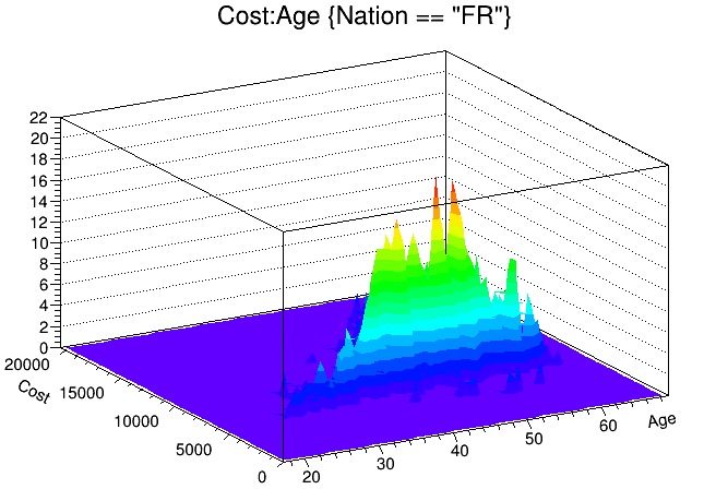
Change the active pad to 3, and add a selection to the list of parameters of the draw command.
This will draw the Costvs. Age for the entries where the nation is equal to “FR”. You can use any C++ operator, and some functions defined in TFormula, in the selection parameter. The value of the selection is used as a weight when filling the histogram. If the expression includes only Boolean operations as in the example above, the result is 0 or 1. If the result is 0, the histogram is not filled. In general, the expression is:
If the Boolean expression evaluates to true, the histogram is filled with a weight. If the weight is not explicitly specified it is assumed to be 1.
For example, this selection will add 1 to the histogram if x is less than y and the square root of z is less than 3.2.
On the other hand, this selection will add x+y to the histogram if the square root of z is larger than 3.2.
The Draw method has its own parser, and it only looks in the current tree for variables. This means that any variable used in the selection must be defined in the tree. You cannot use an arbitrary global variable in the TTree::Draw method.
The TTree::Draw method also accepts TCutG objects. A TCut is a specialized string object used for TTree selections. A TCut object has a name and a title. It does not have any data members in addition to what it inherits from TNamed. It only adds a set of operators to do logical string concatenation. For example, assume:
then
Operators =, +=, +, *, !, &&, || are overloaded, here are some examples:
root[] TCut c1 = "x < 1"
root[] TCut c2 = "y < 0"
root[] TCut c3 = c1 && c2
root[] MyTree.Draw("x", c1)
root[] MyTree.Draw("x", c1 || "x>0")
root[] MyTree.Draw("x", c1 && c2)
root[] MyTree.Draw("x", "(x + y)" * (c1 && c2))The TTree::Draw method creates a histogram called htemp and puts it on the active pad. In a batch program, the histogram htemp created by default, is reachable from the current pad.
   // draw the histogram
   nt->Draw("x", "cuts");
   // get the histogram from the current pad
   TH1F *htemp = (TH1F*)gPad->GetPrimitive("htemp");
   // now we have full use of the histogram
   htemp->GetEntries();
If you pipe the result of the TTree::Draw into a histogram, the histogram is also available in the current directory. You can do:
   // Draw the histogram and fill hnew with it
   nt->Draw("x>>hnew","cuts");
   // get hnew from the current directory
   TH1F *hnew = (TH1F*)gDirectory->Get("hnew");
   // or get hnew from the current Pad
TH1F *hnew = (TH1F*)gPad->GetPrimitive("hnew");The next parameter is the draw option for the histogram:
The draw options are the same as for TH1::Draw. See “Draw Options” where they are listed. In addition to the draw options defined in TH1, there are three more. The 'prof' and 'profs' draw a profile histogram (TProfile) rather than a regular 2D histogram (TH2D) from an expression with two variables. If the expression has three variables, a TProfile2D is generated.
The ‘profs’ generates a TProfile with error on the spread. The ‘prof’ option generates a TProfile with error on the mean. The “goff” option suppresses generating the graphics. You can combine the draw options in a list separated by commas. After typing the lines above, you should now have a canvas that looks this.
When superimposing two 2-D histograms inside a script with TTree::Draw and using the “same” option, you will need to update the pad between Draw commands.
{
   // superimpose two 2D scatter plots
   // Create a 2D histogram and fill it with random numbers
   TH2 *h2 = new TH2D ("h2","2D histo",100,0,70,100,0,20000);
   for (Int_t i = 0; i < 10000; i++)
      h2->Fill(gRandom->Gaus(40,10),gRandom->Gaus(10000,3000));
   // set the color to differentiate it visually
   h2->SetMarkerColor(kGreen);
   h2->Draw();
   // Open the example file and get the tree
   TFile f("cernstaff.root");
   TTree *myTree = (TTree*)f.Get("T");
   // the update is needed for the next draw command to work properly
   gPad->Update();
   myTree->Draw("Cost:Age", "","same");
}
In this example, h2->Draw is only adding the object h2 to the pad’s list of primitives. It does not paint the object on the screen. However, TTree::Draw when called with option “same” gets the current pad coordinates to build an intermediate histogram with the right limits. Since nothing has been painted in the pad yet, the pad limits have not been computed. Calling pad->Update() forces the painting of the pad and allows TTree::Draw to compute the right limits for the intermediate histogram.
There are two more optional parameters to the TTree::Draw method: one is the number of entries and the second one is the entry to start with. For example, this command draws 1000 entries starting with entry 100:
The examples below use the Event.root file generated by the $ROOTSYS/test/Event executable and the Event, Track, and EventHeader class definitions are in $ROOTSYS/test/Event.h. The commands have been tested on the split-levels 0, 1, and 9. Each command is numbered and referenced by the explanations immediately following the examples.
    // Data members and methods
1   tree->Draw("fNtrack");
2   tree->Draw("event.GetNtrack()");
3   tree->Draw("GetNtrack()");
4   tree->Draw("fH.fXaxis.fXmax");
5   tree->Draw("fH.fXaxis.GetXmax()");
6   tree->Draw("fH.GetXaxis().fXmax");
7   tree->Draw("GetHistogram().GetXaxis().GetXmax()");
    // Expressions in the selection parameter
8   tree->Draw("fTracks.fPx","fEvtHdr.fEvtNum%10 == 0");
9   tree->Draw("fPx","fEvtHdr.fEvtNum%10 == 0");
    // Two dimensional arrays defined as:
    //   Float_t fMatrix[4][4] in Event class
10  tree->Draw("fMatrix");
11  tree->Draw("fMatrix[ ][ ]");
12  tree->Draw("fMatrix[2][2]");
13  tree->Draw("fMatrix[ ][0]");
14  tree->Draw("fMatrix[1][ ]");
    // using two arrays... Float_t  fVertex[3];  in Track class
15  tree->Draw("fMatrix - fVertex");
16  tree->Draw("fMatrix[2][1]  - fVertex[5][1]");
17  tree->Draw("fMatrix[ ][1]  - fVertex[5][1]");
18  tree->Draw("fMatrix[2][ ]  - fVertex[5][ ]");
19  tree->Draw("fMatrix[ ][2]  - fVertex[ ][1]");
20  tree->Draw("fMatrix[ ][2]  - fVertex[ ][ ]");
21  tree->Draw("fMatrix[ ][ ]  - fVertex[ ][ ]");
    // variable length arrays
22  tree->Draw("fClosestDistance");
23  tree->Draw("fClosestDistance[fNvertex/2]");
    // mathematical expressions
24  tree->Draw("sqrt(fPx*fPx + fPy*fPy + fPz*fPz))");
    // external function call
25  tree->Draw("TMath::BreitWigner(fPx,3,2)");
    // strings
26  tree->Draw("fEvtHdr.fEvtNum","fType=="type1" ");
27  tree->Draw("fEvtHdr.fEvtNum","strstr(fType,"1" ");
    // Where fPoints is defined in the track class:
    //        Int_t  fNpoint;
    //        Int_t *fPoints; [fNpoint]
28  tree->Draw("fTracks.fPoints");
29  tree->Draw("fTracks.fPoints - fTracks.fPoints[][fAvgPoints]");
30  tree->Draw("fTracks.fPoints[2][]- fTracks.fPoints[][55]");
31  tree->Draw("fTracks.fPoints[][] - fTracks.fVertex[][]");
    // selections
32  tree->Draw("fValid&0x1","(fNvertex>10) && (fNseg<=6000)");
33  tree->Draw("fPx","(fBx>.4) || (fBy<=-.4)");
34  tree->Draw("fPx","fBx*fBx*(fBx>.4) + fBy*fBy*(fBy<=-.4)");
35  tree->Draw("fVertex","fVertex>10");
36  tree->Draw("fPx[600]");
37  tree->Draw("fPx[600]","fNtrack>600");
    // alphanumeric bin histogram
    // where Nation is a char* indended to be used as a string
38  tree->Draw("Nation");
    // where MyByte is a char* intended to be used as a byte
39  tree->Draw("MyByte + 0");
    // where fTriggerBits is a data member of TTrack of type TBits
40  tree->Draw("fTracks.fTriggerBits");
    // using alternate values
41  tree->Draw("fMatrix-Alt$(fClosestDistance,0)");
    // using meta information about the formula
42  tree->Draw("fMatrix:Iteration$")
43 T->Draw("fLastTrack.GetPx():fLastTrack.fPx");
44 T->Scan("((Track*)(fLastTrack@.GetObject())).GetPx()","","");
45 tree->Draw("This->GetReadEntry()");
46  tree->Draw("mybr.mystring");
47 tree->Draw("myTimeStamp");tree->Draw("fNtrack");It fills the histogram with the number of tracks for each entry. fNtrack is a member of event.
tree->Draw("event.GetNtrack()");Same as case 1, but use the method of event to get the number of tracks. When using a method, you can include parameters for the method as long as the parameters are literals.
tree->Draw("GetNtrack()");Same as case 2, the object of the method is not specified. The command uses the first instance of the GetNtrack method found in the objects stored in the tree. We recommend using this shortcut only if the method name is unique.
tree->Draw("fH.fXaxis.fXmax");Draw the data member of a data member. In the tree, each entry has a histogram. This command draws the maximum value of the X-axis for each histogram.
tree->Draw("fH.fXaxis.GetXmax()");Same as case 4, but use the method of a data member.
tree->Draw("fH.GetXaxis().fXmax");The same as case 4: a data member of a data member retrieved by a method.
tree->Draw("GetHistogram().GetXaxis().GetXmax()");Same as case 4, but using methods.
tree->Draw("fTracks.fPx","fEvtHdr.fEvtNum%10 == 0");Use data members in the expression and in the selection parameter to plot fPx or all tracks in every 10th entry. Since fTracks is a TClonesArray of Tracks, there will be d values of fPx for each entry.
tree->Draw("fPx","fEvtHdr.fEvtNum%10 == 0");Same as case 8, use the name of the data member directly.
tree->Draw("fMatrix");When the index of the array is left out or when empty brackets are used [], all values of the array are selected. Draw all values of fMatrix for each entry in the tree. If fMatrix is defined as: Float_t fMatrix[4][4], all 16 values are used for each entry.
tree->Draw("fMatrix[ ][ ]");The same as case 10, all values of fMatrix are drawn for each entry.
tree->Draw("fMatrix[2][2]");The single element at fMatrix[2][2] is drawn for each entry.
tree->Draw("fMatrix[][0]");Four elements of fMatrix are used: fMatrix[1][0], fMatrix[2][0], fMatrix[3][0], fMatrix[4][0].
tree->Draw("fMatrix[1][ ]");Four elements of fMatrix are used: fMatrix[1][0], fMatrix[1][2], fMatrix[1][3], fMatrix[1][4].
tree->Draw("fMatrix - fVertex");With two arrays and unspecified element numbers, the number of selected values is the minimum of the first dimension times the minimum of the second dimension. In this case fVertex is also a two dimensional array since it is a data member of the tracks array. If fVertex is defined in the track class as: Float_t *fVertex[3], it has fNtracks x 3 elements. fMatrix has 4 x 4 elements. This case, draws 4 (the smaller of fNtrack and 4) times 3 (the smaller of 4 and 3), meaning 12 elements per entry. The selected values for each entry are:
fMatrix[0][0] - fVertex[0][0]
fMatrix[0][1] - fVertex[0][1]
fMatrix[0][2] - fVertex[0][2]
fMatrix[1][0] - fVertex[1][0]
fMatrix[1][1] - fVertex[1][1]
fMatrix[1][2] - fVertex[1][2]
fMatrix[2][0] - fVertex[2][0]
fMatrix[2][1] - fVertex[2][1]
fMatrix[2][2] - fVertex[2][2]
fMatrix[3][0] - fVertex[3][0]
fMatrix[3][1] - fVertex[3][1]
fMatrix[3][2] - fVertex[3][2]
tree->Draw("fMatrix[2][1] - fVertex[5][1]");This command selects one value per entry.
tree->Draw("fMatrix[ ][1] - fVertex[5][1]");The first dimension of the array is taken by the fMatrix.
fMatrix[0][1] - fVertex[5][1]
fMatrix[1][1] - fVertex[5][1]
fMatrix[2][1] - fVertex[5][1]
fMatrix[3][1] - fVertex[5][1]
tree->Draw("("fMatrix[2][ ] - fVertex[5][ ]");The first dimension minimum is 2, and the second dimension minimum is 3 (from fVertex). Three values are selected from each entry:
fMatrix[2][0] - fVertex[5][0]
fMatrix[2][1] - fVertex[5][1]
fMatrix[2][2] - fVertex[5][2]
tree->Draw("fMatrix[ ][2] - fVertex[ ][1]")This is similar to case 18. Four values are selected from each entry:
fMatrix[0][2] - fVertex[0][1]
fMatrix[1][2] - fVertex[1][1]
fMatrix[2][2] - fVertex[2][1]
fMatrix[3][2] - fVertex[3][1]
tree->Draw("fMatrix[ ][2] - fVertex[ ][ ]")This is similar to case 19. Twelve values are selected (4x3) from each entry:
fMatrix[0][2] - fVertex[0][0]
fMatrix[0][2] - fVertex[0][1]
fMatrix[0][2] - fVertex[0][2]
fMatrix[1][2] - fVertex[1][0]
fMatrix[1][2] - fVertex[1][1]
fMatrix[1][2] - fVertex[1][2]
fMatrix[2][2] - fVertex[2][0]
fMatrix[2][2] - fVertex[2][1]
fMatrix[2][2] - fVertex[2][2]
fMatrix[3][2] - fVertex[3][0]
fMatrix[3][2] - fVertex[3][1]
fMatrix[3][2] - fVertex[3][2]
tree->Draw("fMatrix[ ][ ] - fVertex[ ][ ]")This is the same as case 15. The first dimension minimum is 4 (from fMatrix), and the second dimension minimum is 3 (from fVertex). Twelve values are selected from each entry.
tree->Draw("fClosestDistance")This event data member fClosestDistance is a variable length array:
Float_t *fClosestDistance; //[fNvertex]
This command selects all elements, but the number per entry depends on the number of vertices of that entry.
tree->Draw("fClosestDistance[fNvertex/2]")With this command the element at fNvertex/2 of the fClosestDistancearray is selected. Only one per entry is selected.
tree->Draw("sqrt(fPx*fPx + fPy*fPy + fPz*fPz)")This command shows the use of a mathematical expression. It draws the square root of the sum of the product.
tree->Draw("TMath::BreitWigner(fPx,3,2)")The formula can contains call to a function that takes numerical arguments and returns a numerical value. The function needs to be declared to the dictionary and need to be available from the global namespace. In particular, global functions and public static member functions can be called.
tree->Draw("fEvtHdr.fEvtNum","fType=="type1" ")You can compare strings, using the symbols == and !=, in the first two parameters of the Draw command (TTreeFormula). In this case, the event number for ‘type1’ events is plotted.
tree->Draw("fEvtHdr.fEvtNum","strstr(fType,"1") ")To compare strings, you can also use strstr. In this case, events having a ‘1’ in fType are selected.
tree->Draw("fTracks.fPoints")If fPoints is a data member of the Track class declared as:
Int_t fNpoint;
Int_t *fPoints; [fNpoint]
The size of the array fPoints varies with each track of each event. This command draws all the value in the fPoints arrays.
tree->Draw("fTracks.fPoints - fTracks.fPoints[][fAvgPoints]");When fAvgPoints is a data member of the Event class, this example selects:
fTracks[0].fPoints[0] - fTracks[0].fPoint[fAvgPoints]
fTracks[0].fPoints[1] - fTracks[0].fPoint[fAvgPoints]
fTracks[0].fPoints[2] - fTracks[0].fPoint[fAvgPoints]
fTracks[0].fPoints[3] - fTracks[0].fPoint[fAvgPoints]
fTracks[0].fPoints[4] - fTracks[0].fPoint[fAvgPoints]
...
fTracks[0].fPoints[max0]- fTracks[0].fPoint[fAvgPoints]
...
fTracks[1].fPoints[0] - fTracks[1].fPoint[fAvgPoints]
fTracks[1].fPoints[1] - fTracks[1].fPoint[fAvgPoints]
fTracks[1].fPoints[2] - fTracks[1].fPoint[fAvgPoints]
fTracks[1].fPoints[3] - fTracks[1].fPoint[fAvgPoints]
fTracks[1].fPoints[4] - fTracks[1].fPoint[fAvgPoints]
...
fTracks[1].fPoints[max1]- fTracks[1].fPoint[fAvgPoints]
...
fTracks[fNtrack-1].fPoints[0] - fTracks[fNtrack-1].fPoint[fAvgPoints]
fTracks[fNtrack-1].fPoints[1] - fTracks[fNtrack-1].fPoint[fAvgPoints]
fTracks[fNtrack-1].fPoints[2] - fTracks[fNtrack-1].fPoint[fAvgPoints]
fTracks[fNtrack-1].fPoints[3] - fTracks[fNtrack-1].fPoint[fAvgPoints]
fTracks[fNtrack-1].fPoints[4] - fTracks[fNtrack-1].fPoint[fAvgPoints]
...
fTracks[fNtrack-1].fPoints[maxn] - fTracks[fNtrack-1].fPoint[fAvgPoints]
Wheremax0, max1, ... max n, is the size of thefPointsarray for the respective track.
tree->Draw("fTracks.fPoints[2][]- fTracks.fPoints[][55]")For each event, this expression is selected:
fTracks[2].fPoints[0] - fTracks[0].fPoints[55]
fTracks[2].fPoints[1] - fTracks[1].fPoints[55]
fTracks[2].fPoints[2] - fTracks[2].fPoints[55]
fTracks[2].fPoints[3] - fTracks[3].fPoints[55]
...
fTracks[2].fPoints[max] - fTracks[max].fPoints[55]
where max is the minimum of fNtrack and fTracks[2].fNpoint.
tree->Draw("fTracks.fPoints[][] - fTracks.fVertex[][]")For each event and each track, this expression is selected. It is the difference between fPoints and of fVertex. The number of elements used for each track is the minimum of fNpoint and 3 (the size of the fVertex array).
fTracks[0].fPoints[0] - fTracks[0].fVertex[0]
fTracks[0].fPoints[1] - fTracks[0].fVertex[1]
fTracks[0].fPoints[2] - fTracks[0].fVertex[2]
// with fTracks[1].fNpoint==7
fTracks[1].fPoints[0] - fTracks[1].fVertex[0]
fTracks[1].fPoints[1] - fTracks[1].fVertex[1]
fTracks[1].fPoints[2] - fTracks[1].fVertex[2]
// with fTracks[1].fNpoint==5
fTracks[2].fPoints[0] - fTracks[2].fVertex[0]
fTracks[2].fPoints[1] - fTracks[2].fVertex[1]
// with fTracks[2].fNpoint==2
fTracks[3].fPoints[0] - fTracks[3].fVertex[0]
// with fTracks[3].fNpoint==1
fTracks[4].fPoints[0] - fTracks[4].fVertex[0]
fTracks[4].fPoints[1] - fTracks[4].fVertex[1]
fTracks[4].fPoints[2] - fTracks[4].fVertex[2]
// with fTracks[4].fNpoint==3
tree->Draw("fValid&0x1","(fNvertex>10) && (fNseg<=6000)")You can use bit patterns (&,|,<<) or Boolean operation.
tree->Draw("fPx","(fBx>.4) || (fBy<=-.4)");
tree->Draw("fPx","fBx*fBx*(fBx>.4) + fBy*fBy*(fBy<=-.4)");
The selection argument is used as a weight. The expression returns a multiplier and in case of a Boolean the multiplier is either 0 (for false) or 1 (for true). The first command draws fPx for the range between with conditions on fBx and fBy, the second command draws fPx for the same conditions, but adds a weight using the result of the second expression.
tree->Draw("fVertex","fVertex>10")When using arrays in the selection and the expression, the selection is applied to each element of the array.
if (fVertex[0]>10) fVertex[0]
if (fVertex[1]>10) fVertex[1]
if (fVertex[2]>10) fVertex[2]
tree->Draw("fPx[600]")
tree->Draw("fPx[600]","fNtrack > 600")
When using a specific element for a variable length array the entries with fewer elements are ignored. Thus these two commands are equivalent.
tree->Draw("Nation")Nation is a char* branch. When drawing a char* it will plot an alphanumeric histogram, of the different value of the string Nation. The axis will have the Nation values. See “Histograms”.
tree->Draw("MyChar +0")If you want to plot a char* variable as a byte rather than a string, you can use the syntax above.
tree->Draw("fTracks.fTriggerBits")fTriggerBits is a data member of TTrack of type TBits. Objects of class TBits can be drawn directly. This command will create a 1D histogram from 0 to nbits which is filled for each non-null bit-number.
tree->Draw("fMatrix-Alt$(fClosestDistance,0)")Alt$(primary,alternate) returns the value of “primary” if it is available for the current iteration; otherwise return the value of “alternate”. Assuming that fClosestDistance is a smaller array than fMatrix. This example will draw fMatrix[i]+fClosestDistance[i] for i less than the size of fClosestDistance, and will draw fMatrix[i]+0 for the other value of i.
tree->Draw("fClosestDistance:Iteration$")This example draws a 2D plot with, for all entries, fClosestDistance[i]:i for each value of i between 0 and the size of fClosestDistance. Iterations$ is one of four special variables giving some indications of the state of the loops implied by the formula:
Entry$ : return the current entry number (TTree::GetReadEntry())
Entries$ : return the total number of entries (TTree::GetEntries())
Length$ : return the total number of element of this formula for this entry
Iteration$: return the current iteration over this formula for this entry (i.e. varies from 0 to Length$).
tree->Draw("fLastTrack.GetPx():fLastTrack.fPx");TRef and TRefArray are automatically deferenced and this shows the value of the fPx of the track referenced by fLastTrack. To access the TRef object itself use the ‘@’ notation (see next example). This auto dereferencing can be extended (via an implementation of TVirtualRefProxy) to any reference type.
tree->Scan("((Track*)(fLastTrack@.GetObject())).GetPx()","","");Will cast the return value of GetObject() (which happens to be TObject* in this case) before requesting the GetPx() member functions.
tree->Draw("This->GetReadEntry()");You can refer to the tree (or chain) containing the data by using the string ‘This’. You can also call any TTree methods. Next example will display the name of the first ‘user info’ object:
tree->Draw("This->GetUserInfo()->At(0)->GetName()");
tree->Draw("mybr.mystring");TString and std::string object are plotted directly. The example 45 draws the same results - i.e. an histogram whose labels are the string value of ‘mystring’:
tree->Draw("mybr.mystring.c_str()");
or
tree->Draw("mybr.mytstring.Data()");
tree->Draw("myTimeStamp");You can plot plot objects of any class which has either AsDouble or AsString (AsDouble has priority). For such a class (for example TTimeStamp), the line 46 will plot the same as:
tree->Draw("myTimeStamp.AsDouble");
AsString can be returning either a char*, or a TString or an std::string.
This section presents the visualization technique available in ROOT to represent multiple variables (>4) data sets.
Spider plots (sometimes called “web-plots” or “radar plots”) are used to compare series of data points (events). They use the human ability to spot un-symmetry.
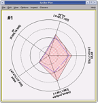
Variables are represented on individual axes displayed along a circle. For each variable the minimum value sits on the circle’s center, and the maximum on the circle’s radius. Spider plots are not suitable for an accurate graph reading since, by their nature, it can be difficult to read out very detailed values, but they give quickly a global view of an event in order to compare it with the others. In ROOT the spider plot facility is accessed from the tree viewer GUI. The variables to be visualized are selected in the tree viewer and can be scanned using the spider plot button.
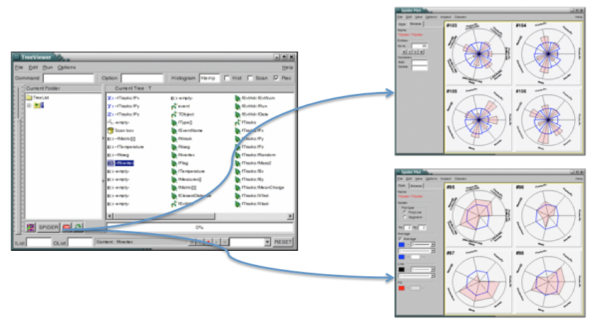
The spider plot graphics editor provides two tabs to interact with the spider plots’ output: the tab “Style” defining the spider layout and the tab “Browse” to navigate in the tree.
The Parallel Coordinates Plots are a common way of studying and visualizing multiple variables data sets. They were proposed by in A.Inselberg in 1981 as a new way to represent multi-dimensional information. In traditional Cartesian coordinates, axes are mutually perpendicular. In Parallel coordinates, all axes are parallel which allows representing data in much more than three dimensions. To show a set of points in Parallel Coordinates, a set of parallel lines is drawn, typically vertical and equally spaced. A point in n-dimensional space is represented as a polyline with vertices on the parallel axes. The position of the vertex on the i-th axis corresponds to the i-th coordinate of the point. The three following figures show some very simple examples:
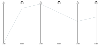
(-5,3,4,2,0,1).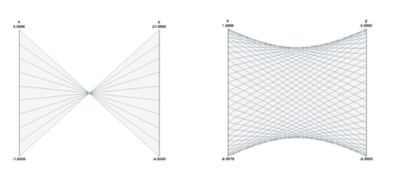
y = -3x+20 and a circle in Parallel Coordinates.The Parallel Coordinates technique is good at: spotting irregular events, seeing the data trend, finding correlations and clusters. Its main weakness is the cluttering of the output. Because each “point” in the multidimensional space is represented as a line, the output is very quickly opaque and therefore it is difficult to see the data clusters. Most of the work done about Parallel Coordinates is to find techniques to reduce the output’s cluttering. The Parallel Coordinates plots in ROOT have been implemented as a new plotting option “PARA” in the TTree::Draw()method. To demonstrate how the Parallel Coordinates works in ROOT we will use the tree produced by the following “pseudo C++” code:
void parallel_example() {
   TNtuple *nt = new TNtuple("nt","Demo ntuple","x:y:z:u:v:w:a:b:c");
   for (Int_t i=0; i<3000; i++) {
      nt->Fill(   rnd,   rnd,   rnd,    rnd,    rnd,    rnd, rnd, rnd, rnd );
      nt->Fill(   s1x,   s1y,   s1z,    s2x,    s2y,    s2z, rnd, rnd, rnd );
      nt->Fill(   rnd,   rnd,   rnd,    rnd,    rnd,    rnd, rnd, s3y, rnd );
      nt->Fill( s2x-1, s2y-1,   s2z, s1x+.5, s1y+.5, s1z+.5, rnd, rnd, rnd );
      nt->Fill(   rnd,   rnd,   rnd,    rnd,    rnd,    rnd, rnd, rnd, rnd );
      nt->Fill( s1x+1, s1y+1, s1z+1,  s3x-2,  s3y-2,  s3z-2, rnd, rnd, rnd );
      nt->Fill(   rnd,   rnd,   rnd,    rnd,    rnd,    rnd, s3x, rnd, s3z );
      nt->Fill(   rnd,   rnd,   rnd,    rnd,    rnd,    rnd, rnd, rnd, rnd );
   }
The data set generated has:
The command used to produce the Parallel Coordinates plot is:
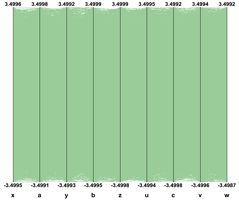
If the 24000 events are plotted as solid lines and no special techniques are used to clarify the picture, the result is the previous picture which is very cluttered and useless. To improve the readability of the Parallel Coordinates output and to explore interactively the data set, many techniques are available. We have implemented a few in ROOT. First of all, in order to show better where the clusters on the various axes are, a 1D histogram is associated to each axis. These histograms (one per axis) are filled according to the number of lines passing through the bins.
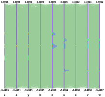
These histograms can be represented which colors (get from a palette according to the bin contents) or as bar charts. Both representations can be cumulated on the same plot. This technique allows seeing clearly where the clusters are on an individual axis but it does not give any hints about the correlations between the axes.
Avery simple technique allows to make the clusters appearing: Instead of painting solid lines we paint dotted lines. The cluttering of each individual line is reduced and the clusters show clearly as we can see on the next figure. The spacing between the dots is a parameter which can be adjusted in order to get the best results.
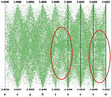
Interactivity is a very important aspect of the Parallel Coordinates plots. To really explore the data set it is essential to act directly with the events and the axes. For instance, changing the axes order may show clusters which were not visible in a different order. On the next figure the axes order has been changed interactively. We can see that many more clusters appear and all the “random spheres” we put in the data set are now clearly visible. Having moved the variables u,v,w after the variables x,y,z the correlation between these two sets of variables is clear also.
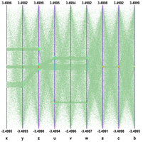
To pursue further data sets exploration we have implemented the possibility to define selections interactively. A selection is a set of ranges combined together. Within a selection, ranges along the same axis are combined with logical OR, and ranges on different axes with logical AND. A selection is displayed on top of the complete data set using its own color. Only the events fulfilling the selection criteria (ranges) are displayed. Ranges are defined interactively using cursors, like on the first axis on the figure. Several selections can be defined at the same time, each selection having its own color.
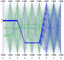
Several selections can been defined. Each cluster is now clearly visible and the zone with crossing clusters is now understandable whereas, without any selection or with only a single one, it was not easy to understand.
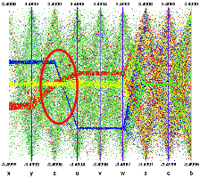
Interactive selections on Parallel Coordinates are a powerful tool because they can be defined graphically on many variables (graphical cuts in ROOT can be defined on two variables only) which allow a very accurate events filtering. Selections allow making precise events choices: a single outlying event is clearly visible when the lines are displayed as “solid” therefore it is easy to make cuts in order to eliminate one single event from a selection. Such selection (to filter one single event) on a scatter plot would be much more difficult.
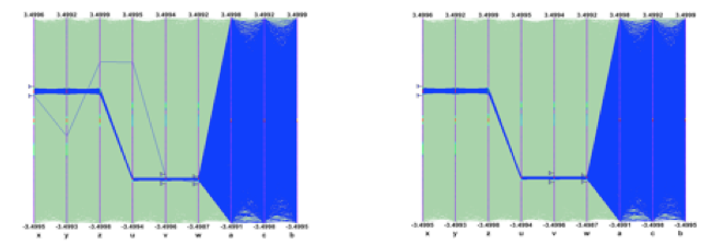
Once a selection has been defined, it is possible to use it to generate a TEntryList which is applied on the tree and used at drawing time. In our example the selection we defined allows to select exactly the two correlated “random spheres”.
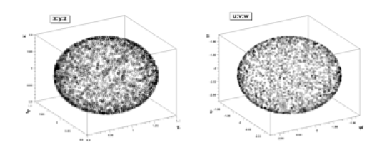
nt->Draw(“x:y:z”) and nt->Draw(“u:v:w”) after applying the selection.Another technique has been implemented in order to show clusters when the picture is cluttered. A weight is assigned to each event. The weight value is computed as: \[ weight = \sum_{i=1}^{n} b_i \]
Where:
The events having the bigger weights are those belonging to clusters. It is possible to paint only the events having a weight above a given value and the clusters appear. The next example “weight cut” applied on the right plot is 50. Only the events with a weight greater than 50 are displayed.
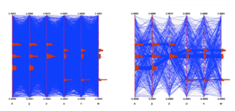
In case only a few events are displayed, drawing them as smooth curves instead of straight lines helps to differentiate them.
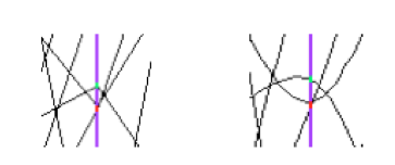
Interactivity and therefore the Graphical User Interface are very important to manipulate the Parallel Coordinates plots. The ROOT framework allows to easily implement the direct interactions on the graphical area and the graphical editor facility provides dedicated GUI.
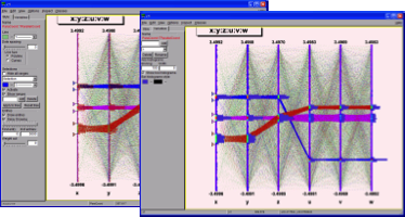
Transparency is very useful with parallel coordinates plots. It allows to show clearly the clusters.
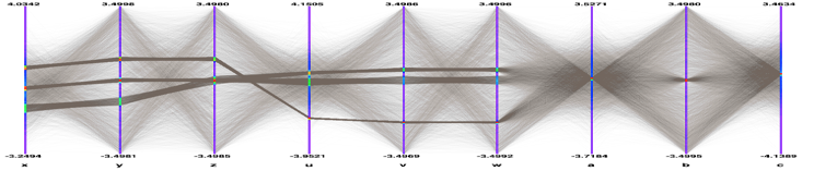
A Box Plot (also known as a “box-and whisker” plot or “candle stick” plot) is a convenient way to describe graphically a data distribution (D) with only the five numbers. It was invented in 1977 by John Tukey. The five numbers are:
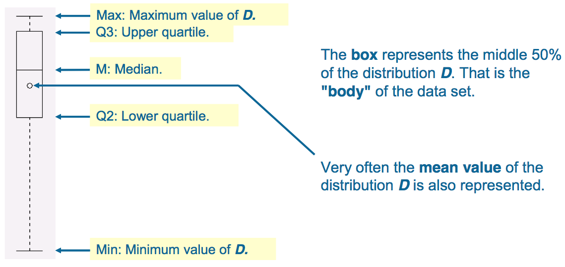
In ROOT Box Plots (Candle Plots) can be produced from a TTree using the “candle” option in TTree::Draw().
TTree::Scan can be used to print the content of the tree’s entries optional passing a selection.
will print the first 8 variables of the tree.
will print all the variable of the tree.
Specific variables of the tree can be explicit selected by list them in column separated list:
will print the values of var1, var2 and var3. A selection can be applied in the second argument:
will print the values of var1, var2 and var3 for the entries where var1 is exactly 0.
TTree::Scan returns the number of entries passing the selection. By default 50 rows are shown before TTree::Scan pauses and ask you to press the Enter key to see the next 50 rows. You can change the default number of rows to be shown before <CR> via mytree->SetScanfield(maxrows) where maxrows is 50 by default. If maxrows is set to 0 all rows of the Tree are shown. This option is interesting when dumping the contents of a Tree to an ascii file, eg from the command line:
will create a file tree.log.
Arrays (within an entry) are printed in their linear forms. If several arrays with multiple dimensions are printed together, they will NOT be synchronized. For example, with a tree containing arr1[4][2]and arr2[2][3],
will results in a printing similar to:
************************************************
*    Row   * Instance *      arr1 *      arr2 *
***********************************************
*        x *        0 * arr1[0][0]* arr2[0][0]*
*        x *        1 * arr1[0][1]* arr2[0][1]*
*        x *        2 * arr1[1][0]* arr2[0][2]*
*        x *        3 * arr1[1][1]* arr2[1][0]*
*        x *        4 * arr1[2][0]* arr2[1][1]*
*        x *        5 * arr1[2][1]* arr2[1][2]*
*        x *        6 * arr1[3][0]*           *
*        x *        7 * arr1[3][1]*           *
However, if there is a selection criterium which is an array, then all the formulas will be synchronized with the selection criterium (see TTree::Draw for more information).
The third parameter of TTree::Scan can be use to specific the layout of the table:
lenmax=dd - where ‘dd’ is the maximum number of elements per array that should be printed. If ‘dd’ is 0, all elements are printed (this is the default).
colsize=ss - where ‘ss’ will be used as the default size for all the column. If this options is not specified, the default column size is 9.
precision=pp - where ‘pp’ will be used as the default ‘precision’ for the printing format.
col=xxx - where ‘xxx’ is colon (:) delimited list of printing format for each column if no format is specified for a column, the default is used.
For example:
will print 3 columns, the first 2 columns will be 30 characters long, the third columns will be 20 characters long. The printf format for the columns (assuming they are numbers) will be respectively: %30.3g %30.3g %20.10g.
The TTree::Drawmethod can also be used to build a list of the entries. When the first argument is preceded by ">>" ROOT knows that this command is not intended to draw anything, but to save the entries in a list with the name given by the first argument. As a result, a TEventList or a TEntryList object is created in the current directory. For example, to create a TEventList of all entries with more than 600 tracks, do:
To create a TEntryList, use the option “entrylist”.
This list contains the entry number of all entries with more than 600 tracks. To see the entry numbers use the Print("all") command.
When using the “>>” whatever was in the list is overwritten. The list can be grown by using the “>>+” syntax. For example to add the entries, with exactly 600 tracks:
If the Draw command generates duplicate entries, they are not added to the list.
This command does not add any new entries to the list because all entries with more than 610 tracks have already been found by the previous command for entries with more than 600 tracks.
The functionality is essentially the same: both are used to store entry numbers. TEntryList, however, uses considerably less memory for storage, and is optimized for both very high and very low selectivity of cuts (see TEntryListBlock class description for the details of internal storage). Unlike the TEventList, TEntryList makes a distinction between indices from a TChain and from a TTree. While a TEntryList for a TTree can be seen as just a list of numbers, a TEntryList for a TChain is a collection of TEntryList(s) for the TTree(s) that constitute this TChain. Such “sub-lists” can be extracted by calling the function
and then be used to construct a new TEntryList for a new TChain, or processed independently as normal TEntryList(s) for TTree(s). This modularity makes TEntryList much better suited for PROOF processing than the TEventList.
A TEventList or a TEntryList can be used to limit the TTree to the events in the list. The methods SetEventList and SetEntryList tell the tree to use the list and hence limit all subsequent calls to Draw, Scan, Process, Query, Principal and CopyTree methods to the entries in the list. In general, it affects the GetEntryNumber method and all functions using it for looping over the tree entries. The GetEntry and GetEntries methods are not affected. Note, that in the SetEventList method, the TEventList argument is internally transformed into a TEntryList, and this operation, in case of a TChain, requires loading of all the tree headers. In this example, we create a list with all entries with more than 600 tracks and then set it so that the tree will use this list. To reset the TTree to use all events use SetEventList(0) or SetEntryList(0).
fNtrack.root[] TFile *f = new TFile("Event.root");
root[] TTree *T = (TTree*)f->Get("T");
root[] T->Draw("fNtrack");TEntryList called myList. We get the list from the current directory and assign it to a variable list.root[] T->Draw(">>myList","fNtrack > 600","entrylist");
root[] TEntryList *list=(TEntryList*)gDirectory->Get("myList");T to use the new list and draw it again. Note that this is exactly the same Draw command. The list limits the entries.You should now see a canvas similar to this one.
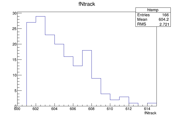
If you have entry lists that were created using different cuts, you can combine the lists to get a new list, with entries passing at least one of the cuts. Example:
root[] T->Draw(">>list1","fNtrack>600","entrylist");
root[] TEntryList *list1 = (TEntryList*)gDirectory->Get("list1");
root[] T->Draw(">>list2","fNtrack<590","entrylist");
root[] TEntryList *list2 = (TEntryList*)gDirectory->Get("list2");
root[] list1->Add(list2);
list1 now contains entries with more than 600 or less than 590 tracks. Check this by calling:
You can also subtract TEntryList from each other, so that the first list contains only the entries, passing the selection of the first list and not present in the second list.
To add some individual entries, use TEntryList::Enter() function. To remove the entries you don’t like, use TEntryList::Remove(). To see if the entry is in the list, use TEntryList::Contains(). Remember, that all operation in a TEntryList for a TChain are on the TTree level. This is illustrated by the following example:
root[] TEntryList *list1 = new TEntryList("list1","list1");
root[] list1->SetTree("tree1","file1")
root[] list1->Enter(0);
root[] list1->Enter(2);
root[] TEntryList *list2 = new TEntryList("list2", "list2");
root[] list2->SetTree("tree2", "file2");
root[] list2->Enter(0);
root[] list2->Enter(3);
root[] list1->Add(list2);
root[] list1->Print("all")
tree1 file1
0
2
tree2 file2
0
3
The result is a TEntryList for a TChain of tree1 and tree2. If the second list was for the same TTree in the same file as the first list, the result would be as follows:
root[] TEntryList *list2_2 = new TEntryList("list2_2", "list2_2");
root[] list2_2->SetTree("tree2", "file2");
root[] list2_2->Enter(1);
root[] list2_2->Enter(2);
root[] list2->Add(list2_2);
root[] list2->Print("all")
tree2 file2
0
1
2
3This is a special kind of TEntryList, used only when processing TChain objects (see the method TChain::SetEntryListFile()). It is used in the case, when the entry lists, corresponding to the trees of this chain, are stored in separate files. It allows to load the entry lists in memory one by one, keeping only the list for the currently processed tree loaded.
For more details on entry lists, see TEntryList, TEntryListBlock and TEntryListFromFile class descriptions, functions TChain::SetEntryList(), TChain::SetEntryListFile(), and the macro $ROOTSYS/test/stressEntryList.C.
The TTree::Draw method can also be used to fill a specific histogram. The syntax is:
root[] TFile *f = new TFile("Event.root")
root[] T->Draw("fNtrack >> myHisto")
root[] myHisto->Print()
TH1.Print Name= myHisto, Entries= 100, Total sum= 100
As we can see, this created a TH1, called myHisto. If you want to append more entries to the histogram, you can use this syntax:
If you do not create a histogram ahead of time, ROOT will create one at the time of the Draw command (as is the case above). If you would like to draw the variable into a specific histogram where you, for example, set the range and bin number, you can define the histogram ahead of time and use it in the Draw command. The histogram has to be in the same directory as the tree.
When you project a TTree into a histogram, the histogram inherits the TTree attributes and not the current style attributes. This allows you to project two Trees with different attributes into the same picture. You can call the method TTree::UseCurrentStyle to change the histogram to use the current style gStyle. See "Graphics and the Graphical User Interface.
The binning of the newly created histogram can be specified in two ways. You can set a default in the .rootrc and/or you can add the binning information in the TTree::Draw command.
To set number of bins default for the 1-D, 2-D, 3-D histograms can be specified in the .rootrc file via the environment variables, e.g.:
# default binnings   Hist.Binning.1D.x: 100

Hist.Binning.2D.x: 40
Hist.Binning.2D.y: 40
Hist.Binning.2D.Prof: 100

Hist.Binning.3D.x: 20
Hist.Binning.3D.y: 20
Hist.Binning.3D.z: 20
Hist.Binning.3D.Profx: 100
Hist.Binning.3D.Profy: 100
To set the number of bins for a specific histogram when using TTree::Draw, add up to nine numbers following the histogram name. The numbers meaning is:
1 bins in x-direction
2 lower limit in x-direction
3 upper limit in x-direction
4-6 same for y-direction
7-9 same for z-direction
When a bin number is specified, the value becomes the default. Any of the numbers can be skipped. For example:
   tree.Draw("sqrt(x)>>hsqrt(500,10,20)";
   // plot sqrt(x) between 10 and 20 using 500 bins
   tree.Draw("sqrt(x):sin(y)>>hsqrt(100,10,,50,.1,.5)";
   // plot sqrt(x) against sin(y) 100 bins in x-direction;
   // lower limit on x-axis is 10; no upper limit
   // 50 bins in y-direction; lower limit on y-axis is .1;
   // upper limit is .5
When the name is followed by binning information, appending the histogram with a “+”, will not reset hsqrt, but will continue to fill it.
This works for 1-D, 2-D and 3-D histograms.
If you would like to fill a histogram, but not draw it you can use the TTree::Project() method.
In case of a two dimensional expression, you can generate a TProfile histogram instead of a two dimensional histogram by specifying the 'prof' or ’profs' option. The prof option is automatically selected when the output is redirected into a TProfile. For example y:x>>pf where pfis an existing TProfile histogram.
Once we have drawn a tree, we can get information about the tree. These are the methods used to get information from a drawn tree TTree:
GetSelectedRows: Returns the number of entries accepted by the selection expression. In case where no selection was specified, it returns the number of entries processed.
GetV1: Returns a pointer to the float array of the first variable.
GetV2: Returns a pointer to the float array of second variable
GetV3: Returns a pointer to the float array of third variable.
GetW: Returns a pointer to the float array of Weights where the weight equals the result of the selection expression.
To read the drawn values of fNtrack into an array, and loop through the entries follow the lines below. First, open the file and draw the fNtrack variable:
Then declare a pointer to a float and use the GetV1 method to retrieve the first dimension of the tree. In this example we only drew one dimension (fNtrack) if we had drawn two, we could use GetV2 to get the second one.
Loop through the first 10 entries and print the values of fNtrack:
root[] for (int i = 0; i < 10; i++)
root[] cout << a[i] << " " << endl   // need an endl to see the values
594 597 606 595 604 610 604 602 603 596
By default, TTree::Draw creates these arrays with fEstimate words where fEstimate can be set via TTree::SetEstimate. If you have more entries than fEstimate only the first fEstimate selected entries will be stored in the arrays. The arrays are used as buffers. When fEstimate entries have been processed, ROOT scans the buffers to compute the minimum and maximum of each coordinate and creates the corresponding histograms. You can use these lines to read all entries into these arrays:
Obviously, this will not work if the number of entries is very large. This technique is useful in several cases, for example if you want to draw a graph connecting all the x, y(or z) points. Note that you may have a tree (or chain) with 1 billion entries, but only a few may survive the cuts and will fit without problems in these arrays.
The TTree::Draw method is convenient and easy to use; however it falls short if you need to do some programming with the variable.
For example, for plotting the masses of all oppositely changed pairs of tracks, you would need to write a program that loops over all events, finds all pairs of tracks, and calculates the required quantities. We have shown how to retrieve the data arrays from the branches of the tree in the previous section, and you could just write that program from scratch. Since this is a very common task, ROOT provides a utility that generates a skeleton class designed to loop over the entries of the tree.
This is the TTree::MakeClass method. We will now go through the steps of using MakeClass with a simplified example. The methods used here obviously work for complex event loop calculations.
These are our assumptions: we would like to do selective plotting and loop through each entry of the tree and tracks. We chose a simple example: we want to plot fPx of the first 100 tracks of each entry. We have a ROOT tree with a branch for each data member in the “Event” object. To build this file and tree follow the instructions on how to build the examples in $ROOTSYS/test. Execute Event and instruct it to split the object with this command (from the UNIX command line).
This creates an Event.root file with 400 events, compressed, split, and filled.
See $ROOTSYS/test/MainEvent.cxx for more info.
The person who designed the tree makes a shared library available to you, which defines the classes needed. In this case, the classes are Event, EventHeader, and Track and they are defined in the shared library libEvent.so. The designer also gives you the Event.h file to see the definition of the classes. You can locate Event.h in $ROOTSYS/test, and if you have not yet built libEvent.so, please see the instructions of how to build it (typing make in $ROOTSYS/test is enough). If you have already built it, you can now use it again.
First, we load the shared library and open Event.root.
root[] .L libEvent.so
root[] TFile *f = new TFile("Event.root");
root[] f->ls();
TFile**         Event.root      TTree benchmark ROOT file
TFile*         Event.root      TTree benchmark ROOT file
KEY: TH1F     htime;1 Real-Time to write versus time
KEY: TTree    T;1     An example of a ROOT tree
We can see there is a tree “T”, and just to verify that we are working with the correct one, we print the tree, which will show us the header and branches.
From the output of print we can see that the tree has one branch for each data member of Event, Track, and EventHeader. Now we can use TTree::MakeClass on our tree “T”. MakeClass takes one parameter, a string containing the name of the class to be made. In the command below, the name of our class will be “MyClass”.
Cling informs us that it has created two files. MyClass.h contains the class definition and MyClass.C contains the MyClass::Loop() method. MyClass has more methods than just Loop(). The other methods are a constructor, a destructor, GetEntry(), LoadTree(), Notify(), Cut() and Show(). The implementations of these methods are in the .h file. This division of methods was done intentionally. The .C file is kept as short as possible, and contains only code that is intended for you to customize. The .h file contains all the other methods. It is clear that you want to be as independent as possible of the header file (i.e. MyClass.h) generated by MakeClass. The solution is to implement a derived class, for example MyRealClass deriving from MyClass such that a change in your Treeor regeneration of MyClass.h does not force you to change MyRealClass.h. You can imagine deriving several classes from MyClass.h, each with a specific algorithm. To understand both files, let’s start with MyClass.h and the class declaration:
class MyClass {
   public :
      // Pointer to the analyzed TTree or TChain
      TTree          *fChain;
      // Current Tree number in a TChain
      Int_t           fCurrent;
      // Declaration of leaves types
      UInt_t          fUniqueID;
      UInt_t          fBits;
      Char_t          fType[20];
      Int_t           fNtrack;
      Int_t           fNseg;
      Int_t           fNvertex;
      UInt_t          fFlag;
      Float_t         fTemperature;
      Int_t           fEvtHdr_fEvtNum;
      // List of branches
      TBranch        *b_fUniqueID;
      TBranch        *b_fBits;
      TBranch        *b_fType;
      TBranch        *b_fNtrack;
      TBranch        *b_fNseg;
      TBranch        *b_fNvertex;
      TBranch        *b_fFlag;
      TBranch        *b_fTemperature;
      TBranch        *b_fEvtHdr_fEvtNum;
...
             MyClass(TTree *tree=0);
            ~MyClass();
      Int_t  Cut(Int_t entry);
      Int_t  GetEntry(Int_t entry);
      Int_t  LoadTree(Int_t entry);
      void   Init(TTree *tree);
      void   Loop();
      Bool_t Notify();
      void   Show(Int_t entry = -1);
};
We can see data members in the generated class. The first data member is fChain. Once this class is instantiated, fChain will point to the original tree or chain this class was made from. In our case, this is “T” in “Event.root”. If the class is instantiated with a tree as a parameter to the constructor, fChain will point to the tree named in the parameter. Next is fCurrent, which is also a pointer to the current tree/chain. Its role is only relevant when we have multiple trees chained together in a TChain. The class definition shows us that this tree has one branch and one leaf per data member. The methods of MyClass are:
MyClass(TTree *tree=0) - this constructor has an optional tree for a parameter. If you pass a tree, MyClass will use it rather than the tree from which it was created.
void Init(TTree *tree) - it is called by the constructor to initialize the tree for reading. It associates each branch with the corresponding leaf data member.
~MyClass() -the destructor, nothing special.
Int_t GetEntry(Int_t entry) - it loads the class with the entry specified. Once you have executed GetEntry, the leaf data members in MyClass are set to the values of the entry. For example, GetEntry(12) loads the 13th event into the event data member of MyClass (note that the first entry is 0). GetEntry returns the number of bytes read from the file. In case the same entry is read twice, ROOT does not have to do any I/O. In this case GetEntry returns 1. It does not return 0, because many people assume a return of 0 means an error has occurred while reading.
Int_t LoadTree(Int_t entry) and void Notify() - these two methods are related to chains. LoadTree will load the tree containing the specified entry from a chain of trees. Notify is called by LoadTree to adjust the branch addresses.
void Loop() - it is the skeleton method that loops through each entry of the tree. This is interesting to us, because we will need to customize it for our analysis.
MyClass::Loop consists of a for-loop calling GetEntry for each entry. In the template, the numbers of bytes are added up, but it does nothing else. If we were to execute it now, there would be no output.
void MyClass::Loop() {
   if (fChain == 0) return;

   Int_t nentries = Int_t(fChain->GetEntries());
   Int_t nbytes = 0, nb = 0;
   for (Int_t jentry=0; jentry<nentries;jentry++) {
      Int_t ientry = LoadTree(jentry);
      // in case of a TChain   , ientry is the entry number in the
      // current file
      nb = fChain->GetEntry(jentry);   nbytes += nb;
      // if (Cut(ientry) < 0) continue;
   }
}
At the beginning of the file are instructions about reading selected branches. They are not reprinted here, but please read them from your own file
Let us continue with the goal of going through the first 100 tracks of each entry and plot Px. To do this we change the Loop method.
...
   if (fChain == 0) return;
   Int_t nentries = Int_t(fChain->GetEntries());
   TH1F *myHisto  = new TH1F("myHisto","fPx", 100, -5,5);
   TH1F *smallHisto = new TH1F("small","fPx", 100, -5,5);
...
In the for-loop, we need to add another for-loop to go over all the tracks. In the outer for-loop, we get the entry and the number of tracks. In the inner for-loop, we fill the large histogram (myHisto) with all tracks and the small histogram (smallHisto) with the track if it is in the first 100.
...
   for (Int_t jentry=0; jentry<nentries;jentry++) {
      GetEntry(jentry);
      for (Int_t j = 0; j < 100; j++) {
         myHisto->Fill(fTracks_fPx[j]);
         if (j < 100) {
            smallHisto->Fill(fTracks_fPx[j]);
         }
      }
   }
...
Outside of the for-loop, we draw both histograms on the same canvas.
Save these changes to MyClass.C and start a fresh root session. We will now load MyClass and experiment with its methods.
The first step is to load the library and the class file. Then we can instantiate a MyClass object.
Now we can get a specific entry and populate the event leaf. In the code snipped below, we get entry 0, and print the number of tracks (594). Then we get entry 1 and print the number of tracks (597).
root[] m.GetEntry(0)
(int)57503
root[] m.fNtrack()
(Int_t)594
root[] m.GetEntry(1)
(int)48045
root[] m.fNtrack()
(Int_t)597
Now we can call the Loop method, which will build and display the two histograms.
You should now see a canvas that looks like this.
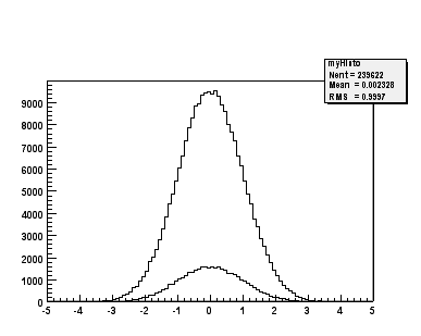
To conclude the discussion on MakeClass let us lists the steps that got us here.
Call TTree::MakeClass, which automatically creates a class to loop over the tree.
Modify the MyClass::Loop() method in MyClass.C to fit your task.
Load and instantiate MyClass, and run MyClass::Loop().
With a TTree we can make a selector and use it to process a limited set of entries. This is especially important in a parallel processing configuration where the analysis is distributed over several processors and we can specify which entries to send to each processor. The TTree::Process method is used to specify the selector and the entries. Before we can use TTree::Process we need to make a selector. We can call the TTree::MakeSelector method. It creates two files similar to TTree::MakeClass.
In the resulting files is a class that is a descendent of TSelector and implements the following methods:
TSelector::Begin() - this method is called every time a loop over the tree starts. This is a convenient place to create your histograms.
TSelector::Notify() - it is called at the first entry of a new tree in a chain.
TSelector::Process() - it is called to process an event. It is the user’s responsibility to read the corresponding entry in memory (may be just a partial read). Once the entry is in memory one can apply a selection and if the event is selected histograms can be filled. Processing stops when this function returns kFALSE. It combines the methods TSelector::ProcessCut() and TSelector::ProcessFill() in one, avoiding the necessity to maintain the state in the class to communicate between these two functions. It reduces the information that needs to be shared between them and promotes a more granular data access by reading branches as they are needed.
TSelector::Terminate() - it is called at the end of a loop on a TTree. This is a convenient place to draw and fit your histograms.
TSelector::Version() - this function provides backward compatibility for old versions and support for the future upgrades.
The TSelector, unlike the resulting class from MakeClass, separates the processing into a ProcessCut() and ProcessFill(), so we can limit reading of branches to the ones we need.
When a selector is used with a TChain in methods Process(), ProcessFill(), ProcessCut(), you must use the pointer to the current TTree to call the method GetEntry(entry). The parameter entry is always the local entry number in the current tree. Assuming that fChain is the pointer to the TChain being processed, use
To create a selector call:
Where T is the TTree and MySelector is the name of created class and the name of the .h and .C files. The resulting TSelector is the argument to TTree::Process. The argument can be the file name or a pointer to the selector object.
This call will interpret the class defined in MySelector.C and process 1000 entries beginning with entry 100. The file name can be appended with a “+” or a “++” to use ACLiC.
When appending a “++”, the class will be compiled and dynamically loaded.
When appending a “+”, the class will also be compiled and dynamically loaded. When it is called again, it recompiles only if the macro (MySelector.C) has changed since it was compiled last. If not, it loads the existing library. The next example shows how to create a selector with a pointer:
Using this form, you can do things like:
   selector->public_attribute1 = init_value;
   for (int i=0; i<limit; i++) {
      T->Process(selector);
      selector->public_attribute1 =
         function(selector->public_attribute2);
   }
TTree::Process() is aware of PROOF, ROOT parallel processing facility. If PROOF is setup, it divides the processing amongst the slave CPUs.
The program $ROOTSYS/test/bench.cxx compares the I/O performance of STL vectors to the ROOT native TClonesArrays collection class. It creates trees with and without compression for the following cases: vector<THit>, vector<THit*>, TClonesArray(TObjHit) not split TClonesArray(TObjHit) split.
The next graphs show the two columns on the right which represent the split and non-split TClonesArray, are significantly lower than the vectors. The most significant difference is in reading a file without compression.
The file size with compression, write times with and without compression and the read times with and without compression all favor the TClonesArray.
This benchmark illustrates the pros and cons of the compression option. We recommend using compression when the time spent in I/O is small compared to the total processing time. In this case, if the I/O operation is increased by a factor of 5 it is still a small percentage of the total time and it may very well save a factor of 10 on disk space. On the other hand if the time spend on I/O is large, compression may slow down the program’s performance. The standard test program $ROOTSYS/test/Event was used in various configurations with 400 events. The data file contains a TTree. The program was invoked with:
TClonesArray) has the data members of the Track class also split into individual buffers.These tests were run on Pentium III CPU with 650 MHz.
| Event Parameters | File Size | Total Time to Write (MB/sec) | Effective Time to Write (MB/sec) | Total Time to Read All (MB/sec) | Total Time to Read Sample (MB/sec) |
Comp = 0 Split = 1 |
19.75 MB | 6.84 s.(2.8 MB/s) | 3.56 s.(5.4 MB/s) | 0.79s.(24.2 MB/s) | 0.79 s.(24.2 MB/s) |
Comp = 1 Split = 1 |
17.73 MB | 6.44 s.(3.0 MB/s) | 4.02 s.(4.8 MB/s) | 0.90 s.(21.3 MB/s) | 0.90 s.(21.3 MB/s) |
Comp = 2 Split = 1 |
13.78 MB | 11.34s.(1.7 MB/s) | 9.51 s.(2.0 MB/s) | 2.17 s.(8.8 MB/s) | 2.17 s.(8.8 MB/s) |
The Total Time is the real time in seconds to run the program. Effective time is the real time minus the time spent in non I/O operations (essentially the random number generator). The program Event generates in average 600 tracks per event. Each track has 17 data members. The read benchmark runs in the interactive version of ROOT. The ‘Total Time to Read All’ is the real time reported by the execution of the script &ROOTSYS/test/eventa.
We did not correct this time for the overhead coming from the interpreter itself. The Total time to read sample is the execution time of the script $ROOTSYS/test/eventb. This script loops on all events. For each event, the branch containing the number of tracks is read. In case the number of tracks is less than 585, the full event is read in memory. This test is obviously not possible in non-split mode. In non-split mode, the full event must be read in memory. The times reported in the table correspond to complete I/O operations necessary to deal with machine independent binary files. On Linux, this also includes byte-swapping operations. The ROOT file allows for direct access to any event in the file and direct access to any part of an event when split=1.
Note also that the uncompressed file generated with split=0 is 48.7 Mbytes and only 47.17 Mbytes for the option split=1. The difference in size is due to the object identification mechanism overhead when the event is written to a single buffer. This overhead does not exist in split mode because the branch buffers are optimized for homogeneous data types. You can run the test programs on your architecture. The program Event will report the write performance. You can measure the read performance by executing the scripts eventa and eventb. The performance depends not only of the processor type, but also of the disk devices (local, NFS, AFS, etc.).
A TChain object is a list of ROOT files containing the same tree. As an example, assume we have three files called file1.root, file2.root, file3.root. Each file contains one tree called “T”. We can create a chain with the following statements:
   TChain chain("T");   // name of the tree is the argument
   chain.Add("file1.root");
   chain.Add("file2.root");
   chain.Add("file3.root");
The name of the TChain will be the same as the name of the tree; in this case it will be "T". Note that twoobjects can have the same name as long as they are not histograms in the same directory, because there, the histogram names are used to build a hash table. The class TChain is derived from the class TTree. For example, to generate a histogram corresponding to the attribute “x” in tree “T” by processing sequentially the three files of this chain, we can use the TChain::Draw method.
When using a TChain, the branch address(es) must be set with:
rather than:
The second form returns the pointer to the branch of the current TTree in the chain, typically the first one. The information is lost when the next TTree is loaded. The following statements illustrate how to set the address of the object to be read and how to loop on all events of all files of the chain.
{
   TChain chain("T"); // create the chain with tree "T"
   chain.Add("file1.root"); // add the files
   chain.Add("file2.root");
   chain.Add("file3.root");
   TH1F *hnseg = new TH1F("hnseg",
                          "Number of segments for selected tracks",
                          5000,0,5000);
   // create an object before setting the branch address
   Event *event = new Event();
   // Specify the address where to read the event object
   chain.SetBranchAddress("event", &event);

   // Start main loop on all events In case you want to read only a few
   // branches, use TChain::SetBranchStatus to activate a branch.
   Int_t nevent = chain.GetEntries();
   for (Int_t i=0;i<nevent;i++) {
      // read complete accepted event in memory
      chain.GetEvent(i);
      // Fill histogram with number of segments
      hnseg->Fill(event->GetNseg());
   }
   // Draw the histogram
   hnseg->Draw();
}ATChain has a list of friends similar to a tree (see TTree::AddFriend). You can add a friend to a chain with the TChain::AddFriend method. With TChain::GetListOfFriends you can retrieve the list of friends. The next example has four chains each has 20 ROOT trees from 20 ROOT files.
   TChain ch("t");    // a chain with 20 trees from 20 files
   TChain ch1("t1");
   TChain ch2("t2");
   TChain ch3("t3");
Now we can add the friends to the first chain.
The parameter is the name of friend chain (the name of a chain is always the name of the tree from which it was created). The original chain has access to all variables in its friends. We can use the TChain::Draw method as if the values in the friends were in the original chain. To specify the chain to use in the Draw method, use:
If the variable name is enough to identify uniquely the variable, you can leave out the chain and/or branch name. For example, this generates a 3-d scatter plot of variable “var” in the TChain ch versus variable v1 inTChain t1 versus variable v2 in TChaint2.
When a TChain::Draw is executed, an automatic call to TTree::AddFriendconnects the trees in the chain. When a chain is deleted, its friend elements are also deleted.
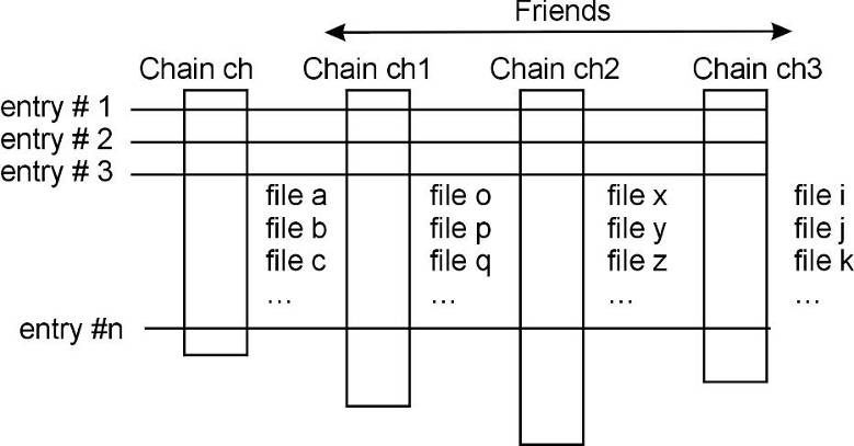
The number of entries in the friend must be equal or greater to the number of entries of the original chain. If the friend has fewer entries a warning is given and the resulting histogram will have missing entries. For additional information see TTree::AddFriends(). A full example of a tree and friends is in Example #3 ($ROOTSYS/tutorials/tree/tree3.C) in the Trees section above.