Unified Histogram Interface (UHI)

ROOT histograms implement the Unified Histogram Interface (UHI), enhancing interoperability with other UHI-compatible libraries. This compliance standardizes histogram operations, making tasks like plotting, indexing, and slicing more intuitive and consistent.

Table of contents

• Plotting
  • Plotting with mplhep
  • Additional Notes
• Indexing
  • Setup
  • Slicing
  • Setting
  • Access
  • Additional Notes

Plotting

ROOT histograms implement the PlottableHistogram protocol. Any plotting library that accepts an object that follows the protocol can plot ROOT histogram objects.

You can read more about the protocol on the UHI plotting page.

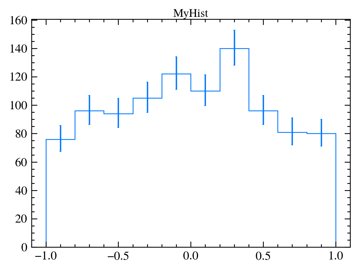
Plotting with mplhep

import ROOT
import matplotlib.pyplot as plt
import mplhep as hep
 
# Create and fill a 1D histogram 
h1 = ROOT.TH1D("h1", "MyHist", 10, -1, 1)
h1.FillRandom("gaus", 1000)
 
# Load a style sheet and plot the histogram
hep.style.use("LHCb2")
hep.histplot(h1)
plt.title("MyHist")
plt.show()

Additional Notes

• UHI plotting related pythonizations are added to all TH1-derived classes (that includes TH2 and TH3).
• While some libraries such as mplhep may not yet support multidimensional PlottableHistogram objects, you can call .values() on your histogram to retrieve a numpy.ndarray and pass it to appropriate plotting functions.
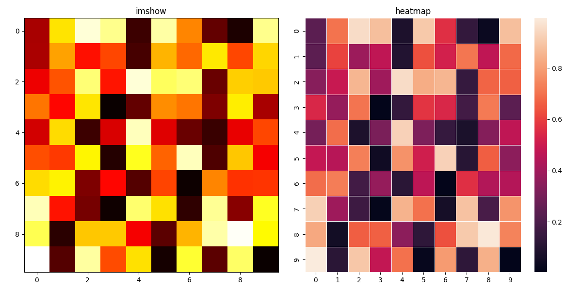
  • Example plotting a 2D ROOT histogram with matplotlib.pyplot.imshow and seaborn.heatmap:

    import ROOT
    import matplotlib.pyplot as plt
    import seaborn as sns
    import numpy as np
     
    h2 = ROOT.TH2D("h2", "h2", 10, -1, 1, 10, -1, 1)
    h2[...] = np.random.rand(10, 10)
     
    fig, (ax1, ax2) = plt.subplots(1, 2, figsize=(12, 6))
     
    # First subplot with imshow
    ax1.imshow(h2.values(), cmap='hot', interpolation='nearest')
    ax1.set_title("imshow")
     
    # Second subplot with seaborn heatmap
    sns.heatmap(h2.values(), linewidth=0.5, ax=ax2)
    ax2.set_title("heatmap")
     
    plt.tight_layout()
    plt.show()

Indexing

ROOT histograms implement the UHI indexing specification. This introduces a unified syntax for accessing and setting bin values, as well as slicing histogram axes.

You can read more about the syntax on the UHI Indexing page.

Setup

The loc, undeflow, overflow, rebin and sum tags are imported from the ROOT.uhi module.

import ROOT
from ROOT.uhi import loc, underflow, overflow, rebin, sum
import numpy as np
 
 
h = ROOT.TH2D("h2", "h2", 10, 0, 1, 10, 0, 1)

Slicing

# Slicing over everything
h == h[:, :]
h == h[...]
 
# Slicing a range, picking the bins 1 to 5 along the x axis and 2 to 6 along the y axis
h1 = h[1:5, 2:6]
 
# Slicing leaving out endpoints
h2 = h[:5, 6:]
 
# Slicing using data coordinates, picking the bins from the one containing the value 0.5 onwards along both axes
h3 = h[loc(0.5):, loc(0.5):]
 
# Combining slicing with rebinning, rebinning the x axis by a factor of 2
h4 = h[1:9:rebin(2), :]

Setting

# Setting the bin contents
h[1, 2] = 5
 
# Setting the bin contents using data coordinates
h[loc(3), loc(1)] = 5
 
# Setting the flow bins
h[overflow, overflow] = 5
 
# Setting the bin contents using a numpy array
h[...] = np.ones((10, 10))
 
# Setting the bin contents using a scalar
h[...] = 5

Access

# Accessing the bin contents using the bin number
v = h[1, 2]
 
# Accessing the bin contents using data coordinates
v = h[loc(0.5), loc(0.5)]
v = h[loc(0.5) + 1, loc(0.5) + 1] # Returns the bin above the one containing the value 2 along both axes
 
# Accessing the flow bins
v = h[underflow, underflow]

Additional Notes

• Indexing system
  • ROOT histograms use a bin indexing system that ranges from 0 to nbins+1 where 0 is the underflow bin and nbins+1 is the overflow (see conventions for numbering bins). In contrast, UHI inherits 0-based indexing from numpy array conventions where 0 is the first valid element and n-1 is the last valid element. Our implementation complies with the UHI conventions by implementing the following syntax:
    • h[underflow] returns the underflow bin (equivalent to h.GetBinContent(0)).
    • h[0] returns the first valid bin (equivalent to h.GetBinContent(1)).
    • h[-1] returns the last valid bin (equivalent to h.GetBinContent(nbins)).
    • h[overflow] returns the overflow bin (equivalent to h.GetBinContent(nbins+1)).
• Slicing operations
  • Slicing always returns a new histogram with the appropriate values copied from the original one according to the input slice.
  • Values outside of the slice range fall into the flow bins.
• Summing operations with sum
  • For a 1D histogram, the integral of the selected slice is returned.
    • ex. ans = h[a:b:sum] --> ans is the integral value.
  • For a 2D or 3D histogram, a new histogram with reduced dimensionality is returned
    • ex. h_projected = h[:, sum, sum] --> h_projected is a 1D histogram representing the y and z projections along the x axis.
• Setting operations
  • Setting with a scalar does not set the flow bins.
  • Setting with an array checks whether the array matches the shape of the histogram with flow bins or the size without flow bins.