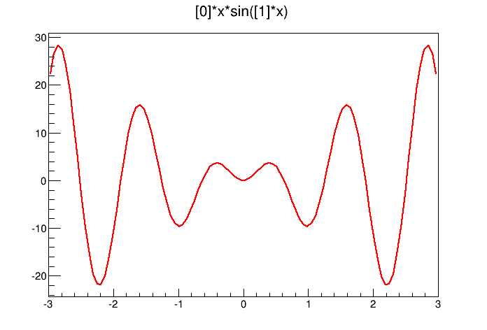
The function x*sin(x)
To fit a histogram you can use the Fit Panel on a visible histogram via the context menu, or you can use the TH1::Fit method. The Fit Panel, which is limited, is best for prototyping. The histogram needs to be drawn in a pad before the Fit Panel is invoked. The method TH1::Fit is more powerful and is used in scripts and programs.
To fit a histogram programmatically, you can use the TH1::Fit method. Here is the signature of TH1::Fit and an explanation of the parameters:
   void Fit(const char *fname, Option_t *option, Option_t *goption,
Axis_t xxmin, Axis_t xxmax)*fname:The name of the fitted function (the model) is passed as the first parameter. This name may be one of ROOT pre-defined function names or a user-defined function. The functions below are predefined, and can be used with the TH1::Fit method:
“gaus” Gaussian function with 3 parameters: f(x) = p0*exp(-0.5*((x-p1)/p2)^2)
“expo”An Exponential with 2 parameters: f(x) = exp(p0+p1*x)
“polN” A polynomial of degree N: f(x) = p0 + p1*x + p2*x2 +...
“landau” Landau function with mean and sigma. This function has been adaptedfrom the CERNLIB routine G110 denlan.
*option:The second parameter is the fitting option. Here is the list of fitting options:
“W” Set all weights to 1 for non empty bins; ignore error bars
“WW” Set all weights to 1 including empty bins; ignore error bars
“I” Use integral of function in bin instead of value at bin center
“L” Use log likelihood method (default is chi-square method)
“U” Use a user specified fitting algorithm
“Q” Quiet mode (minimum printing)
“V” Verbose mode (default is between Q and V)
“E” Perform better errors estimation using the Minos technique
“M” Improve fit results
“R” Use the range specified in the function range
“N” Do not store the graphics function, do not draw
“0” Do not plot the result of the fit. By default the fitted function is drawn unless the option “N” above is specified.
“+” Add this new fitted function to the list of fitted functions (by default, the previous function is deleted and only the last one is kept)
“B”Use this option when you want to fix one or more parameters and the fitting function is like polN, expo, landau, gaus.
“LL”An improved Log Likelihood fit in case of very low statistics and when bincontentsare not integers. Do not use this option if bin contents are large (greater than 100).
“C”In case of linear fitting, don’t calculate the chisquare (saves time).
“F”If fitting a polN, switch to Minuit fitter (by default, polN functions are fitted by the linear fitter).
*goption:The third parameter is the graphics option that is the same as in the TH1::Draw (see the chapter Draw Options).
xxmin, xxmax:Thee fourth and fifth parameters specify the range over which to apply the fit.
By default, the fitting function object is added to the histogram and is drawn in the current pad.
To fit a histogram with a predefined function, simply pass the name of the function in the first parameter of TH1::Fit. For example, this line fits histogram object hist with a Gaussian.
root[] hist.Fit("gaus");The initial parameter values for pre-defined functions are set automatically.
You can create a TF1 object and use it in the call the TH1::Fit. The parameter in to the Fit method is the NAME of the TF1 object. There are three ways to create a TF1.
Using C++ expression using x with a fixed set of operators and functions defined in TFormula.
Same as first one, with parameters
Using a function that you have defined
Let’s look at the first case. Here we call the TF1 constructor by giving it the formula: sin(x)/x.
root[] TF1 *f1 = new TF1("f1","sin(x)/x",0,10)You can also use a TF1 object in the constructor of another TF1.
root[] TF1 *f2 = new TF1("f2","f1*2",0,10)The second way to construct a TF1 is to add parameters to the expression. Here we use two parameters:
root[] TF1 *f1 = new TF1("f1","[0]*x*sin([1]*x)",-3,3);The function x*sin(x)
The parameter index is enclosed in square brackets. To set the initial parameters explicitly you can use:
root[] f1->SetParameter(0,10);This sets parameter 0 to 10. You can also use SetParameters to set multiple parameters at once.
root[] f1->SetParameters(10,5);This sets parameter 0 to 10 and parameter 1 to 5. We can now draw the TF1:
root[] f1->Draw()The third way to build a TF1 is to define a function yourself and then give its name to the constructor. A function for a TF1 constructor needs to have this exact signature:
Double_t fitf(Double_t *x,Double_t *par)The two parameters are:
x a pointer to the dimension array. Each element contains a dimension. For a 1D histogram only x[0] is used, for a 2D histogram x[0] and x[1] is used, and for a 3D histogram x[0], x[1], and x[2] are used. For histograms, only 3 dimensions apply, but this method is also used to fit other objects, for example an ntuple could have 10 dimensions.
par a pointer to the parameters array. This array contains the current values of parameters when it is called by the fitting function.
The following script $ROOTSYS/tutorials/fit/myfit.C illustrates how to fit a 1D histogram with a user-defined function. First we declare the function.
   // define a function with 3 parameters
   Double_t fitf(Double_t *x,Double_t *par) {
      Double_t arg = 0;
      if (par[2]!=0) arg = (x[0] - par[1])/par[2];
      Double_t fitval = par[0]*TMath::Exp(-0.5*arg*arg);
      return fitval;
   }
Now we use the function:
   // this function used fitf to fit a histogram
   void fitexample() {

      // open a file and get a histogram
      TFile *f = new TFile("hsimple.root");
      TH1F *hpx = (TH1F*)f->Get("hpx");

      // Create a TF1 object using the function defined above.
      // The last three parameters specify the number of parameters
      // for the function.
      TF1 *func = new TF1("fit",fitf,-3,3,3);
      // set the parameters to the mean and RMS of the histogram
      func->SetParameters(500,hpx->GetMean(),hpx->GetRMS());

      // give the parameters meaningful names
      func->SetParNames ("Constant","Mean_value","Sigma");

      // call TH1::Fit with the name of the TF1 object
      hpx->Fit("fit");
}Parameters must be initialized before invoking the Fit method. The setting of the parameter initial values is automatic for the predefined functions: poln, exp, gaus, and landau. You can fix one or more parameters by specifying the “B” option when calling the Fit method. When a function is not predefined, the fit parameters must be initialized to some value as close as possible to the expected values before calling the fit function.
To set bounds for one parameter, use TF1::SetParLimits:
func->SetParLimits(0,-1,1);When the lower and upper limits are equal, the parameter is fixed. Next two statements fix parameter 4 at 10.
   func->SetParameter(4,10);
   func->SetParLimits(4,10,10);
However, to fix a parameter to 0, one must call the FixParameter function:
   func->SetParameter(4,0);
   func->FixParameter(4,0);
Note that you are not forced to set the limits for all parameters. For example, if you fit a function with 6 parameters, you can:
   func->SetParameters(0,3.1,1.e-6,-1.5,0,100);
   func->SetParLimits(3,-10,4);
   func->FixParameter(4,0);
With this setup, parameters 0->2 can vary freely, parameter 3 has boundaries [-10, 4] with initial value -1.5, and parameter 4 is fixed to 0.
By default, TH1::Fit will fit the function on the defined histogram range. You can specify the option “R” in the second parameter of TH1::Fit to restrict the fit to the range specified in the TF1 constructor. In this example, the fit will be limited to -3 to 3, the range specified in the TF1 constructor.
root[] TF1 *f1 = new TF1("f1","[0]*x*sin([1]*x)",-3,3);
root[] hist->Fit("f1","R");
You can also specify a range in the call to TH1::Fit:
root[] hist->Fit("f1","","",-2,2)See macros $ROOTSYS/tutorials/fit/myfit.C and multifit.C as more completed examples.
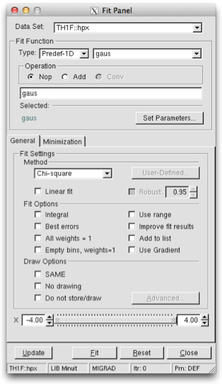
The Fit Panel
To display the Fit Panel right click on a histogram to pop up the context menu, and then select the menu entry Fit Panel.
The new Fit Panel GUI is available in ROOT v5.14. Its goal is to replace the old Fit Panel and to provide more user friendly way for performing, exploring and comparing fits.
By design, this user interface is planned to contain two tabs: “General” and “Minimization”. Currently, the “General” tab provides user interface elements for setting the fit function, fit method and different fit, draw, print options.
The new fit panel is a modeless dialog, i.e. when opened, it does not prevent users from interacting with other windows. Its first prototype is a singleton application. When the Fit Panel is activated, users can select an object for fitting in the usual way, i.e. by left-mouse click on it. If the selected object is suitable for fitting, the fit panel is connected with this object and users can perform fits by setting different parameters and options.
‘Predefined’ combo box - contains a list of predefined functions in ROOT. You have a choice of several polynomials, a Gaussian, a Landau, and an Exponential function. The default one is Gaussian.
‘Operation’ radio button group defines the selected operational mode between functions:
Nop - no operation (default);
Add - addition;
Conv - convolution (will be implemented in the future).
Users can enter the function expression into the text entry field below the ‘Predefined’ combo box. The entered string is checked after the Enter key was pressed and an error message shows up, if the function string is not accepted.
‘Set Parameters’ button opens a dialog for parameters settings, which will be explaned later.
‘Method’ combo box currently provides only two fit model choices: Chi-square and Binned Likelihood. The default one is Chi-square. The Binned Likelihood is recomended for bins with low statistics.
‘Linear Fit’ check button sets the use of Linear fitter when is selected. Otherwise the minimization is done by Minuit, i.e. fit option “F” is applied. The Linear fitter can be selected only for functions linears in parameters (for example - polN).
‘Robust’ number entry sets the robust value when fitting graphs.
‘No Chi-square’ check button switch On/Off the fit option “C” - do not calculate Chi-square (for Linear fitter).
‘Integral’ check button switch On/Off the option “I” - use integral of function instead of value in bin center.
‘Best Errors’ sets On/Off the option “E” - better errors estimation by using Minos technique.
‘All weights = 1’ sets On/Off the option “W”- all weights set to 1 excluding empty bins; error bars ignored.
‘Empty bins, weights=1’ sets On/Off the option “WW” - all weights equal to 1 including empty bins; error bars ignored.
‘Use range’ sets On/Off the option “R” - fit only data within the specified function range. Sliders settings are used if this option is set to On. Users can change the function range values by pressing the left mouse button near to the left/right slider edges. It is possible to change both values simultaneously by pressing the left mouse button near to the slider center and moving it to a new position.
‘Improve fit results’ sets On/Off the option “M”- after minimum is found, search for a new one.
‘Add to list’ sets On/Off the option “+”- add function to the list without deleting the previous one. When fitting a histogram, the function is attached to the histogram’s list of functions. By default, the previously fitted function is deleted and replaced with the most recent one, so the list only contains one function. Setting this option to On will add the newly fitted function to the existing list of functions for the histogram. Note that the fitted functions are saved with the histogram when it is written to a ROOT file. By default, the function is drawn on the pad displaying the histogram.
‘SAME’ sets On/Off function drawing on the same pad. When a fit is executed, the image of the function is drawn on the current pad.
‘No drawing’ sets On/Off the option “0”- do not draw the fit results.
‘Do not store/draw’ sets On/Off option “N”- do not store the function and do not draw it.
This set of options specifies the amount of feedback printed on the root command line after performed fits.
‘Verbose’ - prints fit results after each iteration.
‘Quiet’ - no fit information is printed.
‘Default’ - between Verbose and Quiet.
Fit button - performs a fit taking different option settings via the Fit Panel interface.
Reset - sets the GUI elements and related fit settings to the default ones.
Close - closes the Fit panel window.
The script for this example is $ROOTSYS/tutorials/fit/multifit.C. It shows how to use several Gaussian functions with different parameters on separate sub ranges of the same histogram. To use a Gaussian, or any other ROOT built in function, on a sub range you need to define a new TF1. Each is ‘derived’ from the canned function gaus.
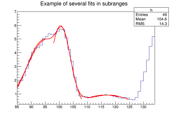
Fitting a histogram with several Gaussian functions
First, four TF1 objects are created - one for each sub-range:
   g1 = new TF1("m1","gaus",85,95);
   g2 = new TF1("m2","gaus",98,108);
   g3 = new TF1("m3","gaus",110,121);
   // The total is the sum of the three, each has 3 parameters
   total = new TF1("mstotal","gaus(0)+gaus(3)+gaus(6)",85,125);
Next, we fill a histogram with bins defined in the array x.
   // Create a histogram and set it's contents
   h = new TH1F("g1","Example of several fits in subranges",
                 np,85,134);
   h->SetMaximum(7);
   for (int i=0; i<np; i++) {
      h->SetBinContent(i+1,x[i]);
   }
   // Define the parameter array for the total function
   Double_t par[9];
When fitting simple functions, such as a Gaussian, the initial values of the parameters are automatically computed by ROOT. In the more complicated case of the sum of 3 Gaussian functions, the initial values of parameters must be set. In this particular case, the initial values are taken from the result of the individual fits. The use of the “+” sign is explained below:
   // Fit each function and add it to the list of functions
   h->Fit(g1,"R");
   h->Fit(g2,"R+");
   h->Fit(g3,"R+");

   // Get the parameters from the fit
   g1->GetParameters(&par[0]);
   g2->GetParameters(&par[3]);
   g3->GetParameters(&par[6]);

   // Use the parameters on the sum
   total->SetParameters(par);
h->Fit(total,"R+");The example $ROOTSYS/tutorials/fit/multifit.C also illustrates how to fit several functions on the same histogram. By default a Fit command deletes the previously fitted function in the histogram object. You can specify the option “+” in the second parameter to add the newly fitted function to the existing list of functions for the histogram.
root[] hist->Fit("f1","+","",-2,2)Note that the fitted function(s) are saved with the histogram when it is written to a ROOT file.
You can combine functions to fit a histogram with their sum as it is illustrated in the macro FitDemo.C ($ROOTSYS/tutorials/fit/FittingDemo.C). We have a function that is the combination of a background and Lorentzian peak. Each function contributes 3 parameters:
\[ y(E) = a_{1} + a_{2}E + a_{3}E^{2} + \frac{A_{p}(\frac{G}{2p})} {(E-m)^{2} + (\frac{G}{2})^2 } \]
BackgroundLorentzian Peak
par[0] = \(a_{1}\) par[0] = \(A_{p}\)
par[1] = \(a_{2}\) par[1] = \(G\)
par[2] = \(a_{3}\) par[2] = \(m\)
The combination function (fitFunction) has six parameters:
fitFunction = background(x,par) + LorentzianPeak(x,&par[3])
par[0]=\(a_{1}\) par[1]=\(a_{2}\) par[2]=\(a_{3}\) par[3]=\(A_{p}\) par[4]=\(G\) par[5]=\(m\)
This script creates a histogram and fits it with the combination of two functions. First we define the two functions and the combination function:
   // Quadratic background function
   Double_t background(Double_t *x, Double_t *par) {
      return par[0] + par[1]*x[0] + par[2]*x[0]*x[0];
   }

   // Lorentzian Peak function
   Double_t lorentzianPeak(Double_t *x, Double_t *par) {
      return (0.5*par[0]*par[1]/TMath::Pi()) / TMath::Max(1.e-10,
      (x[0]-par[2])*(x[0]-par[2])+ .25*par[1]*par[1]);
   }

   // Sum of background and peak function
   Double_t fitFunction(Double_t *x, Double_t *par) {
      return background(x,par) + lorentzianPeak(x,&par[3]);
   }

   void FittingDemo() {
   // bevington exercise by P. Malzacher, modified by R. Brun
   const int nBins = 60;
   Stat_t data[nBins] = {  6, 1,10,12, 6,13,23,22,15,21,
   23,26,36,25,27,35,40,44,66,81,
   75,57,48,45,46,41,35,36,53,32,
   40,37,38,31,36,44,42,37,32,32,
   43,44,35,33,33,39,29,41,32,44,
   26,39,29,35,32,21,21,15,25,15};
   TH1F *histo = new TH1F("example_9_1",
   "Lorentzian Peak on Quadratic Background",60,0,3);

   for(int i=0; i < nBins;  i++) {
      // we use these methods to explicitly set the content
      // and error instead of using the fill method.
      histo->SetBinContent(i+1,data[i]);
      histo->SetBinError(i+1,TMath::Sqrt(data[i]));
   }
   // create a TF1 with the range from 0 to 3 and 6 parameters
   TF1 *fitFcn = new TF1("fitFcn",fitFunction,0,3,6);

   // first try without starting values for the parameters
   // this defaults to 1 for each param.
   histo->Fit("fitFcn");
   // this results in an ok fit for the polynomial function however
   // the non-linear part (Lorentzian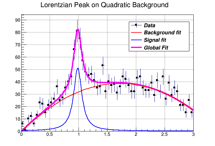
The output of the FittingDemo() example
One or more objects (typically a TF1*) can be added to the list of functions (fFunctions) associated to each histogram. A call to TH1::Fit adds the fitted function to this list. Given a histogram h, one can retrieve the associated function with:
TF1 *myfunc = h->GetFunction("myfunc");If the histogram (or graph) is made persistent, the list of associated functions is also persistent. Retrieve a pointer to the function with the TH1::GetFunction()method. Then you can retrieve the fit parameters from the function (**TF1`**) with calls such as:
root[] TF1 *fit = hist->GetFunction(function_name);
root[] Double_t chi2 = fit->GetChisquare();
// value of the first parameter
root[] Double_t p1 = fit->GetParameter(0);
// error of the first parameter
root[] Double_t e1 = fit->GetParError(0);By default, for each bin, the sum of weights is computed at fill time. One can also call TH1::Sumw2 to force the storage and computation of the sum of the square of weights per bin. If Sumw2 has been called, the error per bin is computed as the sqrt(sum of squares of weights); otherwise, the error is set equal to the sqrt(bin content). To return the error for a given bin number, do:
Double_t error = h->GetBinError(bin);Empty bins are excluded in the fit when using the Chi-square fit method. When fitting the histogram with the low statistics, it is recommended to use the Log-Likelihood method (option ‘L’ or “LL”).
You can change the statistics box to display the fit parameters with the TStyle::SetOptFit(mode) method. This parameter has four digits: mode = pcev (default = 0111)
p = 1 print probabilityc = 1 print Chi-square/number of degrees of freedome = 1 print errors (if e=1, v must be 1)v = 1 print name/values of parametersFor example, to print the fit probability, parameter names/values, and errors, use:
gStyle->SetOptFit(1011);This package was originally written in FORTRAN by Fred James and part of PACKLIB (patch D506). It has been converted to a C++ class by René Brun. The current implementation in C++ is a straightforward conversion of the original FORTRAN version. The main changes are:
The variables in the various Minuit labeled common blocks have been changed to the TMinuit class data members
The internal arrays with a maximum dimension depending on the maximum number of parameters are now data members’ arrays with a dynamic dimension such that one can fit very large problems by simply initializing the TMinuit constructor with the maximum number of parameters
The include file Minuit.h has been commented as much as possible using existing comments in the code or the printed documentation
The original Minuit subroutines are now member functions
Constructors and destructor have been added
Instead of passing the FCN function in the argument list, the addresses of this function is stored as pointer in the data members of the class. This is by far more elegant and flexible in an interactive environment. The member function SetFCN can be used to define this pointer
The ROOT static function Printf is provided to replace all format statements and to print on currently defined output file
The derived class TMinuitOld contains obsolete routines from the FORTRAN based version
The functions SetObjectFit/GetObjectFit can be used inside the FCN function to set/get a referenced object instead of using global variables
By default fGraphicsMode is true. When calling the Minuit functions such as mncont, mnscan, or any Minuit command invoking mnplot, TMinuit::mnplot() produces a TGraph object pointed by fPlot. One can retrieve this object with TMinuit::GetPlot(). For example:
   h->Fit("gaus");
   gMinuit->Command("SCAn 1");
   TGraph *gr = (TGraph*)gMinuit->GetPlot();
   gr->SetMarkerStyle(21);
gr->Draw("alp");Minuit in no graphics mode, call gMinuit->SetGraphicsMode(kFALSE);The Minuit package acts on a multi parameter FORTRAN function to which one must give the generic name FCN. In the ROOT implementation, the function FCN is defined via the Minuit SetFCN member function when a HistogramFit command is invoked. The value of FCN will in general depend on one or more variable parameters.
To take a simple example, in case of ROOT histograms (classes TH1C, TH1S, TH1F, TH1D) the Fit function defines the Minuit fitting function as being H1FitChisquare or H1FitLikelihood depending on the options selected. H1FitChisquare calculates the chi-square between the user fitting function (Gaussian, polynomial, user defined, etc) and the data for given values of the parameters. It is the task of Minuit to find those values of the parameters which give the lowest value of chi-square.
For variable parameters with limits, Minuit uses the following transformation:
Pint = arcsin(2((Pext-a)/(b-a))-1)
Pext = a+((b-a)/(2))(sinPint+1)
so that the internal value Pint can take on any value, while the external value Pext can take on values only between the lower limit a and the ext upper limit b. Since the transformation is necessarily non-linear, it would transform a nice linear problem into a nasty non-linear one, which is the reason why limits should be avoided if not necessary. In addition, the transformation does require some computer time, so it slows down the computation a little bit, and more importantly, it introduces additional numerical inaccuracy into the problem in addition to what is introduced in the numerical calculation of the FCN value. The effects of non-linearity and numerical round off both become more important as the external value gets closer to one of the limits (expressed as the distance to nearest limit divided by distance between limits). The user must therefore be aware of the fact that, for example, if he puts limits of (0, 1010) on a parameter, then the values 0.0 and 1. 0 will be indistinguishable to the accuracy of most machines.
The transformation also affects the parameter error matrix, of course, so Minuit does a transformation of the error matrix (and the ‘’parabolic’’ parameter errors) when there are parameter limits. Users should however realize that the transformation is only a linear approximation, and that it cannot give a meaningful result if one or more parameters is very close to a limit, where \(\frac{\partial Pext}{\partial Pint} \neq 0\). Therefore, it is recommended that:
Limits on variable parameters should be used only when needed in order to prevent the parameter from taking on unphysical values
When a satisfactory minimum has been found using limits, the limits should then be removed if possible, in order to perform or re-perform the error analysis without limits
Minuit offers the user a choice of several minimization algorithms. The MIGRAD algorithm is in general the best minimized for nearly all functions. It is a variable-metric method with inexact line search, a stable metric updating scheme, and checks for positive-definiteness. Its main weakness is that it depends heavily on knowledge of the first derivatives, and fails miserably if they are very inaccurate.
If parameter limits are needed, in spite of the side effects, then the user should be aware of the following techniques to alleviate problems caused by limits:
If MIGRAD converges normally to a point where no parameter is near one of its limits, then the existence of limits has probably not prevented Minuit from finding the right minimum. On the other hand, if one or more parameters is near its limit at the minimum, this may be because the true minimum is indeed at a limit, or it may be because the minimized has become ‘’blocked’’ at a limit. This may normally happen only if the parameter is so close to a limit (internal value at an odd multiple of \(\pm \frac{\pi}{2}\) that Minuit prints a warning to this effect when it prints the parameter values. The minimized can become blocked at a limit, because at a limit the derivative seen by the minimized \(\frac{\partial F}{\partial Pint}\) is zero no matter what the real derivative \(\frac{\partial F}{\partial Pext}\) is.
\[ \left(\frac{\partial F}{\partial Pint}\right) = \left(\frac{\partial F}{\partial Pext}\right) \left(\frac{\partial Pext}{\partial Pint}\right) = \left(\frac{\partial F}{\partial Pext}\right) = 0 \]
In the best case, where the minimum is far from any limits, Minuit will correctly transform the error matrix, and the parameter errors it reports should be accurate and very close to those you would have got without limits. In other cases (which should be more common, since otherwise you would not need limits), the very meaning of parameter errors becomes problematic. Mathematically, since the limit is an absolute constraint on the parameter, a parameter at its limit has no error, at least in one direction. The error matrix, which can assign only symmetric errors, then becomes essentially meaningless.
There are two kinds of problems that can arise: the reliability of Minuit’s error estimates, and their statistical interpretation, assuming they are accurate.
For discussion of basic concepts, such as the meaning of the elements of the error matrix, or setting of exact confidence levels see the articles:
F.James. Determining the statistical Significance of experimental Results. Technical Report DD/81/02 and CERN Report 81-03, CERN, 1981
W.T.Eadie, D.Drijard, F.James, M.Roos, and B.Sadoulet. Statistical Methods in Experimental Physics. North-Holland, 1971
Minuit always carries around its own current estimates of the parameter errors, which it will print out on request, no matter how accurate they are at any given point in the execution. For example, at initialization, these estimates are just the starting step sizes as specified by the user. After a HESSE step, the errors are usually quite accurate, unless there has been a problem. Minuit, when it prints out error values, also gives some indication of how reliable it thinks they are. For example, those marked CURRENT GUESS ERROR are only working values not to be believed, and APPROXIMATE ERROR means that they have been calculated but there is reason to believe that they may not be accurate.
If no mitigating adjective is given, then at least Minuit believes the errors are accurate, although there is always a small chance that Minuit has been fooled. Some visible signs that Minuit may have been fooled:
Warning messages produced during the minimization or error analysis
Failure to find new minimum
Value of EDM too big (estimated Distance to Minimum)
Correlation coefficients exactly equal to zero, unless some parameters are known to be uncorrelated with the others
Correlation coefficients very close to one (greater than 0.99). This indicates both an exceptionally difficult problem, and one which has been badly parameterized so that individual errors are not very meaningful because they are so highly correlated
Parameter at limit. This condition, signaled by a Minuit warning message, may make both the function minimum and parameter errors unreliable. See the discussion above ‘Getting the right parameter errors with limits’
The best way to be absolutely sure of the errors is to use ‘’independent’‘calculations and compare them, or compare the calculated errors with a picture of the function. Theoretically, the covariance matrix for a’‘physical’’ function must be positive-definite at the minimum, although it may not be so for all points far away from the minimum, even for a well-determined physical problem. Therefore, if MIGRAD reports that it has found a non-positive-definite covariance matrix, this may be a sign of one or more of the following:
On its way to the minimum, MIGRAD may have traversed a region that has unphysical behavior, which is of course not a serious problem as long as it recovers and leaves such a region.
If the matrix is not positive-definite even at the minimum, this may mean that the solution is not well defined, for example that there are more unknowns than there are data points, or that the parameterization of the fit contains a linear dependence. If this is the case, then Minuit (or any other program) cannot solve your problem uniquely. The error matrix will necessarily be largely meaningless, so the user must remove the under determinedness by reformulating the parameterization. Minuit cannot do this itself.
It is possible that the apparent lack of positive-definiteness is due to excessive round off errors in numerical calculations (in the user function), or not enough precision. This is unlikely in general, but becomes more likely if the number of free parameters is very large, or if the parameters are badly scaled (not all of the same order of magnitude), and correlations are large. In any case, whether the non-positive-definiteness is real or only numerical is largely irrelevant, since in both cases the error matrix will be unreliable and the minimum suspicious.
For questions of parameter dependence, see the discussion above on positive-definiteness. Possible other mathematical problems are the following:
Excessive numerical round off - be especially careful of exponential and factorial functions which get big very quickly and lose accuracy.
Starting too far from the solution - the function may have unphysical local minima, especially at infinity in some variables.
FUMILI is used to minimize Chi-square function or to search maximum of likelihood function. Experimentally measured values \(F_{i}\) are fitted with theoretical functions \(f_{i}(\vec{x_{i}},\vec{\theta})\), where \(\vec{x_{i}}\) are coordinates, and \(\vec{\theta}\) - vector of parameters. For better convergence Chi-square function has to be the following form
\[ \frac{\chi^2}{2} = \frac{1}{2} \sum_{i=1}^{n} \left(\frac{f_{i}(\vec{x_{i}},\vec{\theta}) - F_{i}} {\sigma_{i}}\right)^{2} \]
where \(\sigma_{i}\) are errors of the measured function. The minimum condition is:
\[ \frac{\partial \chi^{2}}{\partial \theta_{i}} = \sum_{j=1}^{n} \frac{1}{\sigma_{j}^{2}} . \frac{\partial f_{i}}{\partial \theta_{i}} \left[ (\vec{x_{j}},\vec{\theta}) - F_{j}\right] = 0, i = 1 ... m \]
where \(m\) is the quantity of parameters. Expanding left part of this equation over parameter increments and retaining only linear terms one gets
\[ \left(\frac{\partial \chi^{2}}{\theta_{i}}\right) _{\theta = \vec{\theta}^{0}} + \sum_{k} \left(\frac{\partial^{2} \chi^{2}}{\partial \theta_{i} \partial \theta_{k}}\right) _{\theta = \vec{\theta}^{0}} . (\theta_{k} - \theta_{k}^{0}) = 0 \]
here \(\vec{\theta}^{0}\) is some initial value of parameters. In general case:
\[ {\partial^2\chi^2\over\partial\theta_i\partial\theta_k}= \sum^n_{j=1}{1\over\sigma^2_j} {\partial f_j\over\theta_i} {\partial f_j\over\theta_k} + \sum^n_{j=1}{(f_j - F_j)\over\sigma^2_j}\cdot {\partial^2f_j\over\partial\theta_i\partial\theta_k} \]
In FUMILI algorithm for second derivatives of Chi-square approximate expression is used when last term in previous equation is discarded. It is often done, not always wittingly, and sometimes causes troubles, for example, if user wants to limit parameters with positive values by writing down \(\theta_i^2\) instead of \(\theta_i\). FUMILI will fail if one tries minimize \(\chi^2 = g^2(\vec\theta)\) where g is arbitrary function.
Approximate value is:
\[ {\partial^2\chi^2\over\partial\theta_i\partial\theta_k}\approx Z_{ik}= \sum^n_{j=1}{1\over\sigma^2_j}{\partial f_j\over\theta_i} {\partial f_j\over\theta_k} \]
Then the equations for parameter increments are:
\[ \left(\partial\chi^2\over\partial\theta_i\right)_ {\vec\theta={\vec\theta}^0} +\sum_k Z_{ik}\cdot(\theta_k-\theta^0_k) = 0, \qquad i=1\ldots m \]
Remarkable feature of algorithm is the technique for step restriction. For an initial value of parameter \({\vec\theta}^0\) a parallelepiped \(P_0\) is built with the center at \({\vec\theta}^0\) and axes parallel to coordinate axes \(\theta_i\). The lengths of parallelepiped sides along i-th axis is \(2b_i\), where \(b_i\) is such a value that the functions \(f_j(\vec\theta)\) are quasi-linear all over the parallelepiped.
FUMILI takes into account simple linear inequalities in the form:
\[ \theta_i^{\rm min}\le\theta_i\le\theta^{\rm max}_i\]
They form parallelepiped \(P\) (\(P_0\) may be deformed by \(P\)). Very similar step formulae are used in FUMILI for negative logarithm of the likelihood function with the same idea - linearization of function argument.
Neural Networks are used in various fields for data analysis and classification, both for research and commercial institutions. Some randomly chosen examples are image analysis, financial movements’ predictions and analysis, or sales forecast and product shipping optimization. In particles physics neural networks are mainly used for classification tasks (signal over background discrimination). A vast majority of commonly used neural networks are multilayer perceptrons. This implementation of multilayer perceptrons is inspired from the MLPfit package, which remains one of the fastest tools for neural networks studies.
The multilayer perceptron is a simple feed-forward network with the following structure showed on the left.
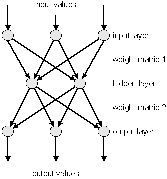
It is made of neurons characterized by a bias and weighted links in between - let’s call those links synapses. The input neurons receive the inputs, normalize them and forward them to the first hidden layer. Each neuron in any subsequent layer first computes a linear combination of the outputs of the previous layer. The output of the neuron is then function of that combination with f being linear for output neurons or a sigmoid for hidden layers.
Such a structure is very useful because of two theorems:
1- A linear combination of sigmoids can approximate any continuous function.
2- Trained with output=1 for the signal and 0 for the background, the approximated function of inputs X is the probability of signal, knowing X.
The aim of all learning methods is to minimize the total error on a set of weighted examples. The error is defined as the sum in quadrate, divided by two, of the error on each individual output neuron. In all methods implemented in this library, one needs to compute the first derivative of that error with respect to the weights. Exploiting the well-known properties of the derivative, one can express this derivative as the product of the local partial derivative by the weighted sum of the outputs derivatives (for a neuron) or as the product of the input value with the local partial derivative of the output neuron (for a synapse). This computation is called “back-propagation of the errors”. Six learning methods are implemented.
This is the most trivial learning method. The Robbins-Monro stochastic approximation is applied to multilayer perceptrons. The weights are updated after each example according to the formula:
\[ w_{ij}(t+1) = w_{ij}(t) + \Delta w_{ij}(t) \]
with:
\[ \Delta w_{ij}(t) = - \eta \left( \frac{\partial e_p}{\partial w_{ij}} + \delta \right) + \epsilon \Delta w_{ij}(t-1) \]
The parameters for this method are Eta, EtaDecay, Delta and Epsilon.
It is the same as the stochastic minimization, but the weights are updated after considering all the examples, with the total derivative dEdw. The parameters for this method are Eta, EtaDecay, Delta and Epsilon.
Weights are set to the minimum along the line defined by the gradient. The only parameter for this method is Tau. Lower Tau = higher precision = slower search. A value Tau=3 seems reasonable.
Weights are set to the minimum along the line defined by the conjugate gradient. Parameters are Tau and Reset, which defines the epochs where the direction is reset to the steepest descent (estimated by using the Polak-Ribiere formula).
Weights are set to the minimum along the line defined by the conjugate gradient. Parameters are Tau and Reset, which defines the epochs where the direction is reset to the steepest descent (estimated by using the Fletcher-Reeves formula).
It implies the computation of a NxN matrix, but seems more powerful at least for less than 300 weights. Parameters are Tau and Reset, which defines the epochs where the direction is reset to the steepest descent.
Neural network are build from a set of “samples”. A sample is a set of values defining the inputs and the corresponding output that the network should ideally provide. In ROOT this is a TTree entry. The first thing to be decided is the network layout. This layout is described in a string where the layers are separated by semicolons. The input/output layers are defined by giving the expression for each neuron, separated by comas. Hidden layers are just described by the number of neurons.
In addition, input and output layer formulas can be preceded by ‘@’ (e.g. “@out”) if one wants to normalize the corresponding value. Also, if the string ends with ‘!’, output neurons are set up for classification, i.e. with a sigmoid (1 neuron) or softmax (more neurons) activation function.
Many questions on the good usage of neural network, including rules of dumb to determine the best network topology are addressed at ftp://ftp.sas.com/pub/neural/FAQ.html
   // a simple network: 2 inputs, 10 hidden and 1 normalized
   // output neuron
   TMultiLayerPerceptron network("r,z:10:@Br",tree);
Expressions are evaluated as for TTree::Draw(). Input and outputs are taken from the TTree associated with the network. This TTree can be given as argument of the constructor or defined later with TMultiLayerPerceptron::SetData(). Events can also be weighted. The weight expression can be given in the constructor or set later with the method SetWeight() of the class TMultiLayerPerceptron. Two datasets must be defined before learning the network: a training dataset that is used when minimizing the error, and a test dataset that will avoid bias. Those two datasets can be build aside and then given to the network, or can be build from a standard expression. By default, half of the events are put in both datasets.
   // a more complex 4:8:1 network
   // the ptsumf branch is used as weigh;
   // default event lists are explicit
   TMultiLayerPerceptron  network("m,pt,acol,acopl:8:type","pt",tree,
                                  "Entry$%2","Entry$/2");
The method TMultiLayerPerceptron::SetLearningMethod() defines the learning method. Learning methods are:
TMultiLayerPerceptron::kStochastic,
TMultiLayerPerceptron::kBatch,
TMultiLayerPerceptron::kSteepestDescent,
TMultiLayerPerceptron::kRibierePolak,
TMultiLayerPerceptron::kFletcherReeves,
TMultiLayerPerceptron::kBFGS      // default
The training can start with TMultiLayerPerceptron::Train(Int_t nepoch,Option_t* options). The first argument is the number of epochs while option is a string that can contain “text” (simple text output), “graph” (evaluating graphical training curves), “update = X” (step for the text/graph output update) or “+” (will skip the randomization and start from the previous values). All combinations are available.
   network.Train(1000,"text,graph,update=10"); // full output every
                                               // 10 epochs
   network.Train(100,"text,+");                // 100 more epochs
   //starts with existing weights
The weights can be saved to a file (DumpWeights) and then reloaded (LoadWeights) to a new compatible network. The output can also be evaluated (Evaluate) for a given output neuron and an array of double input parameters or the network can be exported (Export) as a standalone code. Up to now, this is only as a C++ or PYTHON class, but other languages could be implemented.
An example of how to use TMultiLayerPerceptron is the macro mlpHiggs.C in $ROOTSYS/tutorials. Using some standard simulated information that could have been obtained at LEP, a neural network is build, which can make the difference between WW events and events containing a Higgs boson. Starting with a TFile containing two TTrees: one for the signal, the other for the background, a simple script is used:
   void mlpHiggs(Int_t ntrain=100) {
      if (!gROOT->GetClass("TMultiLayerPerceptron"))
      gSystem->Load("libMLP");
      // prepare inputs - the 2 trees are merged into one, and a
      // "type" branch, equal to 1 for the signal and 0 for the
      // background is added
      TFile input("mlpHiggs.root");
      TTree *signal = (TTree *)input.Get("sig_filtered");
      TTree *background = (TTree *)input.Get("bg_filtered");
      TTree *simu = new TTree("MonteCarlo",
                              "Filtered Monte Carlo Events");
      ...
Since the input is a TTree and we are starting from two different TTrees (with different names), they are first merged into one, and a “type” branch is added, that says whether there is a signal or a background event. Those irrelevant details are skipped here.
      ...
      TMultiLayerPerceptron *mlp = new TMultiLayerPerceptron(
            "msumf,ptsumf, acolin, acopl:8:type","ptsumf",simu,
            "Entry$%2","Entry$/2");
      mlp->Train(ntrain, "text,graph,update=10");
The neural network is instantiated and trained. “ptsumf” is used as a weight, and the standard event lists are explicit. The network that is then build has four input neurons, eight additional ones in the only hidden layer and one single output neuron.
      // Use the NN to plot the results for each sample
      TH1F *bg = new TH1F("bgh","NN output",50,-.5,1.5);
      TH1F *sig = new TH1F("sigh","NN output",50,-.5,1.5);
      bg->SetDirectory(0);
      sig->SetDirectory(0);
      Double_t params[4];
      for (i = 0; i < background->GetEntries(); i++) {
         background->GetEntry(i);
         params[0] = msumf;    params[1] = ptsumf;
         params[2] = acolin;   params[3] = acopl;
         bg->Fill(mlp->Evaluate(0,params));
      }
      for (i = 0; i < signal->GetEntries(); i++) {
         signal->GetEntry(i);
         params[0] = msumf;
         params[1] = ptsumf;
         params[2] = acolin;
         params[3] = acopl;
         sig->Fill(mlp->Evaluate(0,params));
      }
      TCanvas *cv = new TCanvas("NNout_cv","Neural net output");
      bg->SetFillStyle(3008);
      bg->SetFillColor(kBlue);
      sig->SetFillStyle(3003);
      sig->SetFillColor(kRed);
      bg->SetStats(0);
      sig->SetStats(0);
      bg->Draw();
      sig->Draw("same");
      TLegend *legend = new TLegend(.75,.80,.95,.95);
      legend->AddEntry(bg,"Background(WW)");
      legend->AddEntry(sig,"Signal(Higgs)");
      legend->Draw();
The neural net output is then used to display the final difference between background and signal events. The figure “The neural net output” shows this plot.
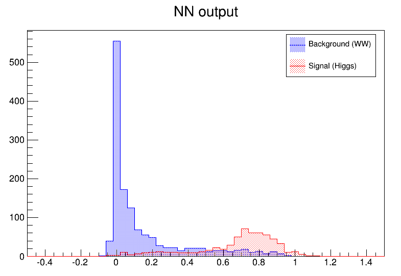
The neural net output
As it can be seen, this is a quite efficient technique. As mentioned earlier, neural networks are also used for fitting function. For some application with a cylindrical symmetry, a magnetic field simulation gives as output the angular component of the potential vector A, as well as the radial and z components of the B field.
One wants to fit those distributions with a function in order to plug them into the Geant simulation code. Polynomial fits could be tried, but it seems difficult to reach the desired precision over the full range. One could also use a spline interpolation between known points. In all cases, the resulting field would not be C-infinite.
An example of output (for Br) is shown. First the initial function can be seen as the target. Then, the resulting (normalized) neural net output. In order to ease the learning, the “normalize output” was used here. The initial amplitude can be recovered by multiplying by the original RMS and then shifting by the original mean.
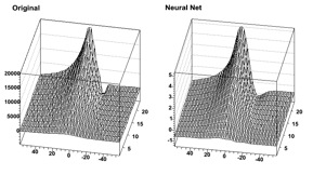
The original and the neural net for Br