WARNING: This documentation is not maintained anymore. Some part might be obsolete or wrong, some part might be missing but still some valuable information can be found there. Instead please refer to the ROOT Reference Guide and the ROOT Manual. If you think some information should be imported in the ROOT Reference Guide or in the ROOT Manual, please post your request to the ROOT Forum or via a Github Issue.
% Chapter: Geometry ________________________________________________________________________________________ WARNING: This documentation is not maintained anymore. Some part might be obsolete or wrong, some part might be missing but still some valuable information can be found there. Instead please refer to the ROOT Reference Guide and the ROOT Manual. If you think some information should be imported in the ROOT Reference Guide or in the ROOT Manual, please post your request to the ROOT Forum or via a Github Issue.
% Chapter: Geometry ________________________________________________________________________________________ WARNING: This documentation is not maintained anymore. Some part might be obsolete or wrong, some part might be missing but still some valuable information can be found there. Instead please refer to the ROOT Reference Guide and the ROOT Manual. If you think some information should be imported in the ROOT Reference Guide or in the ROOT Manual, please post your request to the ROOT Forum or via a Github Issue.
The new ROOT geometry package is a tool for building, browsing, navigating and visualizing detector geometries. The code works standalone with respect to any tracking Monte-Carlo engine; therefore, it does not contain any constraints related to physics. However, the navigation features provided by the package are designed to optimize particle transport through complex geometries, working in correlation with simulation packages such as GEANT3, GEANT4 and FLUKA.
This chapter will provide a detailed description on how to build valid geometries as well as the ways to optimize them. There are several components gluing together the geometrical model, but for the time being let us get used with the most basic concepts.
The basic bricks for building-up the model are called volumes.These represent the un-positioned pieces of the geometry puzzle. The difference is just that the relationship between the pieces is not defined by neighbors, but by containment. In other words, volumes are put one inside another making an in-depth hierarchy. From outside, the whole thing looks like a big pack that you can open finding out other smaller packs nicely arranged waiting to be opened at their turn. The biggest one containing all others defines the “world” of the model. We will often call this master reference system (MARS). Going on and opening our packs, we will obviously find out some empty ones, otherwise, something is very wrong… We will call these leaves (by analogy with a tree structure).
On the other hand, any volume is a small world by itself - what we need to do is to take it out and to ignore all the rest since it is a self-contained object. In fact, the modeller can act like this, considering a given volume as temporary MARS, but we will describe this feature later on. Let us focus on the biggest pack - it is mandatory to define one. Consider the simplest geometry that is made of a single box. Here is an example on how to build it:
We first need to load the geometry library. This is not needed if one does make map in root folder.
Second, we have to create an instance of the geometry manager class. This takes care of all the modeller components, performing several tasks to insure geometry validity and containing the user interface for building and interacting with the geometry. After its creation, the geometry manager class can be accessed with the global gGeoManager:
We want to create a single volume in our geometry, but since any volume needs to have an associated medium, we will create a dummy one. You can safely ignore the following lines for the time being, since materials and media will be explained in detail later on.
root[] TGeoMaterial *mat = new TGeoMaterial("Vacuum",0,0,0);
root[] TGeoMedium   *med = new TGeoMedium("Vacuum",1,mat);
We can finally make our volume having a box shape. Note that the world volume does not need to be a box - it can be any other shape. Generally, boxes and tubes are the most recommendable shapes for this purpose due to their fast navigation algorithms.
The default units are in centimeters. Now we want to make this volume our world. We have to do this operation before closing the geometry.
This should be enough, but it is not since always after defining some geometry hierarchy, TGeo needs to build some optimization structures and perform some checks. Note the messages posted after the statement is executed. We will describe the corresponding operations later.
Now we are really done with geometry building stage, but we would like to see our simple world:
root[] top->SetLineColor(kMagenta);
root[] gGeoManager->SetTopVisible(); // the TOP is invisible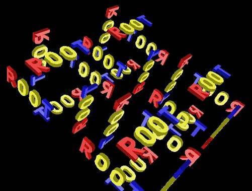
root[] top->Draw();Before going further, let us get a look and feel of interacting with the modeller. For this, we will use one of the examples illustrating the geometry package. To get an idea on the geometry structure created in this example, just look at the link: http://root.cern.ch/root/html/tutorials/visualisation/geom/rootgeom.C.html. You will notice that this is a bit more complex that just creating the “world” since several other volumes are created and put together in a hierarchy. The purpose here is just to learn how to interact with a geometry that is already built, but just few hints on the building steps in this example might be useful. The geometry here represents the word ROOT that is replicated in some symmetric manner. You might for instance ask some questions after having a first look:
Q: “OK, I understand the first lines that load the libGeom library and create a geometry manager object. I also recognize from the previous example the following lines creating some materials and media, but what about the geometrical transformations below?”
A: As explained before, the model that we are trying to create is a hierarchy of volumes based on containment. This is accomplished by positioning some volumes inside others. Any volume is an un-positioned object in the sense that it defines only a local frame (matching the one of its shape). In order to fully define the mother-daughter relationship between two volumes one has to specify how the daughter will be positioned inside. This is accomplished by defining a local geometrical transformation of the daughter with respect to the mother coordinate system. These transformations will be subsequently used in the example.
Q: “I see the lines defining the top level volume as in the previous example, but what about the other volumes named REPLICA and ROOT?”
A: You will also notice that several other volumes are created by using lines like:
TGeoVolume *someVolume = gGeoManager->MakeXXX("someName",
ptrMedium, /* parameters coresponding to XXX ...*/)
In the method above XXX represent some shape name (Box, Tube, etc.). This is just a simple way of creating a volume having a given shape in one-step (see also section: “Creating and Positioning Volumes”). As for REPLICA and ROOT volumes, they are just some virtual volumes used for grouping and positioning together other real volumes. See “Positioned Volumes (Nodes)”. The same structure represented by (a real or) a virtual volume can be replicated several times in the geometry.
Q: “Fine, so probably the real volumes are the ones composing the letters R, O and T. Why one have to define so many volumes to make an R?”
A: Well, in real life some objects have much more complex shapes that an R. The modeller cannot just know all of them; the idea is to make a complex object by using elementary building blocks that have known shapes (called primitive shapes). Gluing these together in the appropriate way is the user responsibility.
Q: “I am getting the global picture but not making much out of it… There are also a lot of calls to TGeoVolume::AddNode() that I do not understand.”
A: A volume is positioned inside another one by using this method. The relative geometrical transformation as well as a copy number must be specified. When positioned, a volume becomes a node of its container and a new object of the class TGeoNode is automatically created. This method is therefore the key element for the creation of a hierarchical link between two volumes. As it will be described further on in this document, there are few other methods performing similar actions, but let us keep things simple for the time being. In addition, notice that there are some visualization-related calls in the example followed by a final TGeoVolume::Draw()call for the top volume. These are explained in details in the section “Visualization Settings and Attributes”. At this point, you will probably like to see how this geometry looks like. You just need to run the example and you will get the following picture that you can rotate using the mouse; or you can zoom / move it around (see what the Help menu of the GL window displays).
Now let us browse the hierarchy that was just created. Start a browser and double-click on the item simple1 representing the gGeoManager object. Note that right click opens the context menu of the manager class where several global methods are available.
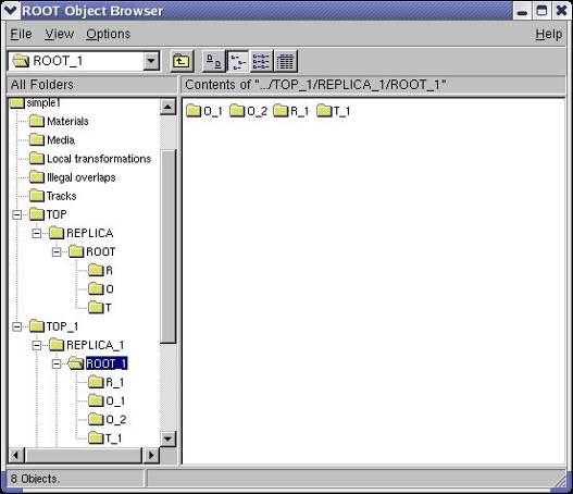
The folders Materials, Media and Local transformations are in fact the containers where the geometry manager stores the corresponding objects. The Illegal overlaps folder is empty but can be filled after performing a geometry validity check (see section: “Checking the Geometry”). If tracking is performed using TGeo, the folder Tracks might contain user-defined tracks that can be visualized/animated in the geometry context (see section: “Creating and Visualizing Tracks”). Since for the time being we are interested more in the geometrical hierarchy, we will focus on the last two displayed items TOPand TOP_1. These are the top volume and the corresponding top node in the hierarchy.
Double clicking on the TOP volume will unfold all different volumes contained by the top volume. In the right panel, we will see all the volumes contained by TOP (if the same is positioned 4 times we will get 4 identical items). This rule will apply to any clicked volume in the hierarchy. Note that right clicking a volume item activates the volume context menu containing several specific methods. We will call the volume hierarchy developed in this way as the logical geometry graph. The volume objects are nodes inside this graph and the same volume can be accessed starting from different branches.
On the other hand, the real geometrical objects that are seen when visualizing or tracking the geometry are depicted in the TOP_1 branch. These are the nodes of the physical tree of positioned volumes represented by TGeoNode objects. This hierarchy is a tree since a node can have only one parent and several daughters. For a better understanding of the hierarchy, have a look at https://root.cern.ch/doc/master/classTGeoManager.html.
Just close now the X3D window and focus at the wire frame picture drawn in a pad. Activate Options/Event Status. Moving the mouse in the pad, you will notice that objects are sometimes changing color to red. Volumes are highlighted in this way whenever the mouse pointer is close enough to one of its vertices. When this happens, the corresponding volume is selected and you will see in the bottom right size of the ROOT canvas its name, shape type and corresponding path in the physical tree. Right clicking on the screen when a volume is selected will also open its context menu (picking). Note that there are several actions that can be performed both at view (no volume selected) and volume level.
TView (mouse not selecting any volume):
SetParallel ()/SetPerspective () - switch from parallel to perspective view.ShowAxis() - show coordinate axes.Centered/Left/Side/Top - change view direction.TGeoVolume (mouse selecting a volume):
CheckOverlaps() - run overlap checker on current volume.Draw () - draw that volume according current global visualization optionsDrawOnly()-draw only the selected volume.InspectShape/Material() - print info about shape or material.Raytrace() - initiate a ray tracing algorithm on current view.RandomPoints/Rays() - shoot random points or rays inside the bounding box of the clicked volume and display only those inside visible volumes.Weight() - estimates the weight of a volume within a given precision.Note that there are several additional methods for visibility and line attributes settings.
We have mentioned that volumes are the building blocks for geometry, but they describe real objects having well defined properties. In fact, there are just two of them: the material they are made from and their geometrical shape. These have to be created before creating the volume itself, so we will describe the bits and pieces needed for making the geometry before moving to an architectural point of view.
As far as materials are concerned, they represent the physical properties of the solid from which a volume is made. Materials are just a support for the data that has to be provided to the tracking engine that uses this geometry package. Due to this fact, the TGeoMaterial class is more like a thin data structure needed for building the corresponding native materials of the Monte-Carlo tracking code that uses TGeo.
In order to make easier material and mixture creation, one can use the pre-built table of elements owned by TGeoManager class:
TGeoElementTable *table = gGeoManager->GetElementTable();
TGeoElement *element1 = table->GetElement(Int_t Z);
TGeoElement *element2 = table->FindElement("Copper");
Materials made of single elements can be defined by their atomic mass (A), charge (Z) and density (rho). One can also create a material by specifying the element that it is made of. Optionally the radiation and absorption lengths can be also provided; otherwise they can be computed on-demand [G3]. The class representing them is TGeoMaterial:
TGeoMaterial(const char *name,Double_t a,Double_t z,
    Double_t density, Double_t radlen=0,Double_t intlen=0);
TGeoMaterial(const char *name, TGeoElement *elem,
    Double_t density);
TGeoMaterial(const char* name, Double_t a, Double_t z,
    Double_t rho,
    TGeoMaterial::EGeoMaterialState state,
    Double_t temperature = STP_temperature,
    Double_t pressure = STP_pressure)
Any material or derived class is automatically indexed after creation. The assigned index is corresponding to the last entry in the list of materials owned by TGeoManager class. This can be changed using the TGeoMaterial::SetIndex() method, however it is not recommended while using the geometry package interfaced with a transport MC. Radiation and absorption lengths can be set using:
radlen: radiation length. If radlen<=0 the value is computed using GSMATE algorithm in GEANT3intlen: absorption lengthMaterial state, temperature and pressure can be changed via setters. Another material property is transparency. It can be defined and used while viewing the geometry with OpenGL.
transparency: between 0 (opaque default) to 100 (fully transparent)One can attach to a material a user-defined object storing Cerenkov properties. Another hook for material shading properties is currently not in use. Mixtures are materials made of several elements. They are represented by the class TGeoMixture, deriving from TGeoMaterial and defined by their number of components and the density:
Elements have to be further defined one by one:
void TGeoMixture::DefineElement(Int_t iel,Double_t a,Double_t z,
    Double_t weigth);
void TGeoMixture::DefineElement(Int_t iel, TGeoElement *elem,
    Double_t weight);
void TGeoMixture::DefineElement(Int_t iel, Int_t z, Int_t natoms);
or:
void AddElement(TGeoMaterial* mat, Double_t weight);
void AddElement(TGeoElement* elem, Double_t weight);
void AddElement(TGeoElement* elem, Int_t natoms);
void AddElement(Double_t a, Double_t z, Double_t weight)
iel: index of the element[0,nel-1]a and z: the atomic mass and chargeweight: proportion by mass of the elementsnatoms: number of atoms of the element in the molecule making the mixtureThe radiation length is automatically computed when all elements are defined. Since tracking MC provide several other ways to create materials/mixtures, the materials classes are likely to evolve as the interfaces to these engines are being developed. Generally in the process of tracking material properties are not enough and more specific media properties have to be defined. These highly depend on the MC performing tracking and sometimes allow the definition of different media properties (e.g. energy or range cuts) for the same material.
A new class TGeoElementRN was introduced in this version to provide support for radioactive nuclides and their decays. A database of 3162 radionuclides can be loaded on demand via the table of elements (TGeoElementTable class). One can make then materials/mixtures based on these radionuclides and use them in a geometry
root[] TGeoManager *geom = new TGeoManager("geom","radionuclides");
root[] TGeoElementTable *table = geom->GetElementTable();
root[] TGeoElementRN *c14 = table->GetElementRN(14,6);  // A,Z
root[] c14->Print();
6-C-014 ENDF=60140; A=14; Z=6; Iso=0; Level=0[MeV]; Dmass=3.0199[MeV];
Hlife=1.81e+11[s]  J/P=0+; Abund=0; Htox=5.8e-10; Itox=5.8e-10; Stat=0
Decay modes:
BetaMinus            Diso:   0 BR:   100.000% Qval: 0.1565
One can make materials or mixtures from radionuclides:
The following properties of radionuclides can be currently accessed via getters in the TGeoElementRN class:
Atomic number and charge (from the base class TGeoElement)
ISO)ENDF=10000*Z+100*A+ISOMeV]MeV]s]TGeoElementRN::GetTitle()TGeoElementRN::GetDecays()The radioactive decays of a radionuclide are represented by the class TGeoDecayChannel and they are stored in a TObjArray. Decay provides:
Q value for the decay [GeV]Radionuclides are linked one to each other via their decays, until the last element in the decay chain which must be stable. One can iterate decay chains using the iterator TGeoElemIter:
root[] TGeoElemIter next(c14);
root[] TGeoElementRN *elem;
root[] while ((elem=next())) next.Print();
6-C-014 (100% BetaMinus) T1/2=1.81e+11
7-N-014 stable
To create a radioactive material based on a radionuclide, one should use the constructor:
To create a radioactive mixture, one can use radionuclides as well as stable elements:
TGeoMixture(const char *name, Int_t nelements, Double_t density);
TGeoMixture::AddElement(TGeoElement *elem,
    Double_t weight_fraction);
Once defined, one can retrieve the time evolution for the radioactive materials/mixtures by using one of the next two methods:
TGeoMaterial::FillMaterialEvolution(TObjArray *population, Double_t precision=0.001)To use this method, one has to provide an empty TObjArray object that will be filled with all elements coming from the decay chain of the initial radionuclides contained by the material/mixture. The precision represent the cumulative branching ratio for which decay products are still considered.
The population list may contain stable elements as well as radionuclides, depending on the initial elements. To test if an element is a radionuclide:
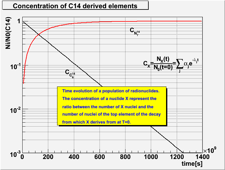
All radionuclides in the output population list have attached objects that represent the time evolution of their fraction of nuclei with respect to the top radionuclide in the decay chain. These objects (Bateman solutions) can be retrieved and drawn:
Another method allows to create the evolution of a given radioactive material/mixture at a given moment in time:
TGeoMaterial::DecayMaterial(Double_t time, Double_t precision=0.001)The method will create the mixture that result from the decay of a initial material/mixture at time, while all resulting elements having a fractional weight less than precision are excluded.
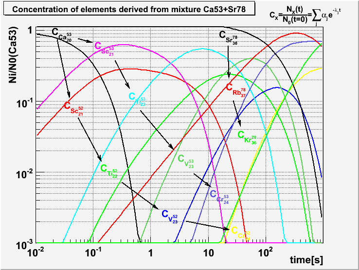
A demo macro for radioactive material features is $ROOTSYS/tutorials/visualisation/geom/RadioNuclides.C It demonstrates also the decay of a mixture made of radionuclides.
The class TGeoMedium describes tracking media properties. This has a pointer to a material and the additional data members representing the properties related to tracking.
name: name assigned to the mediummat: pointer to a materialparams: array of additional parametersAnother constructor allows effectively defining tracking parameters in GEANT3 style:
TGeoMedium(const char *name,Int_t numed,Int_t imat,Int_t ifield,
Double_t fieldm,Double_t tmaxfd,Double_t stemax,
Double_t deemax,Double_t epsil,Double_t stmin);
This constructor is reserved for creating tracking media from the VMC interface […]:
numed: user-defined medium indeximat: unique ID of the materialothers: see G3 documentationLooking at our simple world example, one can see that for creating volumes one needs to create tracking media before. The way to proceed for those not interested in performing tracking with external MC’s is to define and use only one dummy tracking medium as in the example (or a NULL pointer).
The TGeoManager class contains the API for accessing and handling defined materials:
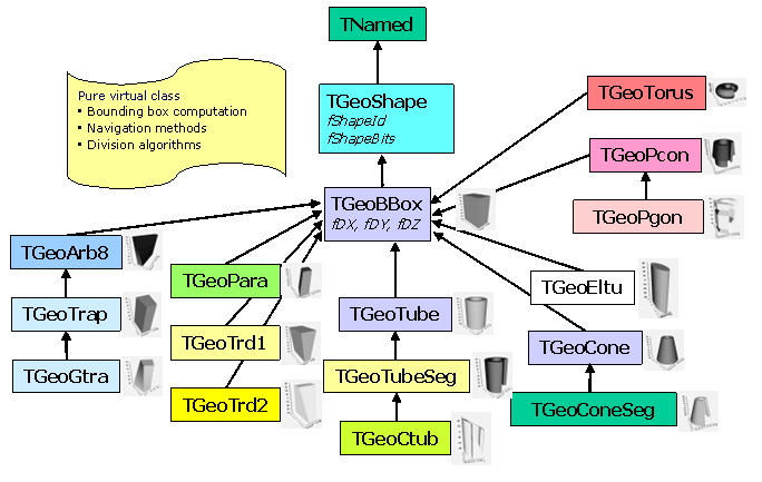
Shapes are geometrical objects that provide the basic modeling functionality. They provide the definition of the local coordinate system of the volume. Any volume must have a shape. Any shape recognized by the modeller has to derive from the base TGeoShape class, providing methods for:
All the features above are globally managed by the modeller in order to provide navigation functionality. In addition to those, shapes have also to implement additional specific abstract methods:
The modeller currently provides a set of 20 basic shapes, which we will call primitives. It also provides a special class allowing the creation of shapes as a result of Boolean operations between primitives. These are called composite shapes and the composition operation can be recursive (combined composites). This allows the creation of a quite large number of different shape topologies and combinations. You can have a look and run the tutorial: http://root.cern.ch/root/html/examples/geodemo.C.html
Shapes are named objects and all primitives have constructors like:
TGeoXXX(const char *name,<type> param1,<type> param2, ...);
TGeoXXX(<type> param1,<type> param2, ...);
Naming shape primitive is mandatory only for the primitives used in Boolean composites (see “Composite Shapes”). For the sake of simplicity, we will describe only the constructors in the second form.
The length units used in the geometry are arbitrary. However, there are certain functionalities that work with the assumption that the used lengths are expressed in centimeters. This is the case for shape capacity or volume weight computation. The same is valid when using the ROOT geometry as navigator for an external transport MC package (e.g. GEANT) via the VMC interface.
Other units in use: All angles used for defining rotation matrices or some shape parameters are expressed in degrees. Material density is expressed in [g/cm3].
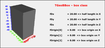
Normally a box has to be built only with 3 parameters: DX,DY,DZ representing the half-lengths on X, Y and Z-axes. In this case, the origin of the box will match the one of its reference frame and the box will range from: -DX to DX on X-axis, from -DY to DY on Y and from -DZ to DZ on Z. On the other hand, any other shape needs to compute and store the parameters of their minimal bounding box. The bounding boxes are essential to optimize navigation algorithms. Therefore all other primitives derive from TGeoBBox. Since the minimal bounding box is not necessary centered in the origin, any box allows an origin translation (Ox,Oy,Oz). All primitive constructors automatically compute the bounding box parameters. Users should be aware that building a translated box that will represent a primitive shape by itself would affect any further positioning of other shapes inside. Therefore it is highly recommendable to build non-translated boxes as primitives and translate/rotate their corresponding volumes only during positioning stage.
A parallelepiped is a shape having 3 pairs of parallel faces out of which one is parallel with the XY plane (Z faces). All faces are parallelograms in the general case. The Z faces have 2 edges parallel with the X-axis.
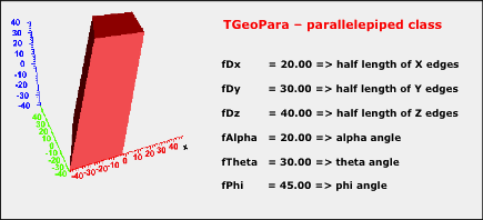
The shape has the center in the origin and it is defined by:
dX, dY, dZ: half-lengths of the projections of the edges on X, Y and Z. The lower Z face is positioned at -dZ, while the upper at +dZ.alpha: angle between the segment defined by the centers of the X-parallel edges and Y axis [-90,90] in degreestheta: theta angle of the segment defined by the centers of the Z faces;phi: phi angle of the same segmentA box is a particular parallelepiped having the parameters: (dX,dY,dZ,0.,0.,0.).
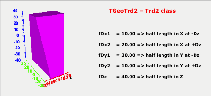
In general, we will call trapezoidal shapes having 8 vertices and up to 6 trapezoid faces. Besides that, two of the opposite faces are parallel to XY plane and are positioned at dZ. Since general trapezoids are seldom used in detector geometry descriptions, there are several primitives implemented in the modeller for particular cases.
Trd1 is a trapezoid with only X varying with Z. It is defined by the half-length in Z, the half-length in X at the lowest and highest Z planes and the half-length in Y:

Trd2 is a trapezoid with both X and Y varying with Z. It is defined by the half-length in Z, the half-length in X at the lowest and highest Z planes and the half-length in Y at these planes:
A general trapezoid is one for which the faces perpendicular to z are trapezes but their centers are not necessary at the same x, y coordinates.
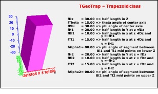
It has eleven parameters: the half length in z, the polar angles from the center of the face at low z to that at high z, H1 the half length in y at low z, LB1 the half length in x at low z and y low edge, LB2 the half length in x at low z and y high edge, TH1 the angle with respect to the y axis from the center of low y edge to the center of the high y edge, and H2,LB2,LH2,TH2, the corresponding quantities at high z.
TGeoTrap(Double_t dz,Double_t theta,Double_t phi,
Double_t h1,Double_t bl1,Double_t tl1,Double_t alpha1,
Double_t h2,Double_t bl2,Double_t tl2,Double_t alpha2);A twisted trapezoid is a general trapezoid defined in the same way but that is twisted along the Z-axis. The twist is defined as the rotation angle between the lower and the higher Z faces.
TGeoGtra(Double_t dz,Double_t theta,Double_t phi,Double_t twist,
Double_t h1,Double_t bl1,Double_t tl1,Double_t alpha1,
Double_t h2,Double_t bl2,Double_t tl2,Double_t alpha2 );
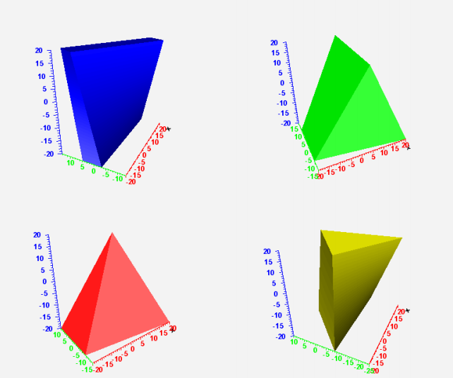
An Arb8 is defined by two quadrilaterals sitting on parallel planes, at dZ. These are defined each by 4 vertices having the coordinates (Xi,Yi,+/-dZ),i=0,3. The lateral surface of the Arb8 is defined by the 4 pairs of edges corresponding to vertices (i,i+1) on both -dZ and +dZ. If M and M’ are the middles of the segments (i,i+1) at -dZ and +dZ, a lateral surface is obtained by sweeping the edge at -dZ along MM’ so that it will match the corresponding one at +dZ. Since the points defining the edges are arbitrary, the lateral surfaces are not necessary planes - but twisted planes having a twist angle linear-dependent on Z.
dz: half-length in Z;ivert = [0,7]Vertices have to be defined clockwise in the XY pane, both at +dz and -dz. The quadrilateral at -dz is defined by indices [0,3], whereas the one at +dz by vertices [4,7]. The vertex with index=7 has to be defined last, since it triggers the computation of the bounding box of the shape. Any two or more vertices in each Z plane can have the same (X,Y) coordinates. It this case, the top and bottom quadrilaterals become triangles, segments or points. The lateral surfaces are not necessary defined by a pair of segments, but by pair segment-point (making a triangle) or point-point (making a line). Any choice is valid as long as at one of the end-caps is at least a triangle.
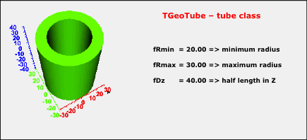
Tubes have Z as their symmetry axis. They have a range in Z, a minimum and a maximum radius:
The full Z range is from -dz to +dz.
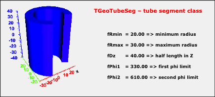
A tube segment is a tube having a range in phi. The tube segment class derives from TGeoTube, having 2 extra parameters: phi1 and phi2.
Here phi1 and phi2are the starting and ending phivalues in degrees. The general phi convention is that the shape ranges from phi1 to phi2 going counterclockwise. The angles can be defined with either negative or positive values. They are stored such that phi1 is converted to [0,360] and phi2 > phi1.
The cut tubes constructor has the form:
TGeoCtub(Double_t rmin,Double_t rmax,Double_t dz,
Double_t phi1,Double_t phi2,
Double_t nxlow,Double_t nylow,Double_t nzlow, Double_t nxhi,
Double_t nyhi,Double_t nzhi);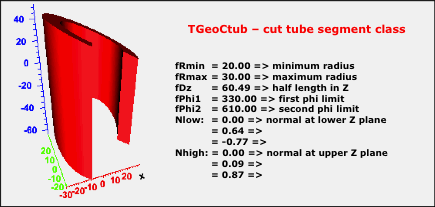
A cut tube is a tube segment cut with two planes. The centers of the 2 sections are positioned at dZ. Each cut plane is therefore defined by a point (0,0,dZ) and its normal unit vector pointing outside the shape:
Nlow=(Nx,Ny,Nz<0), Nhigh=(Nx',Ny',Nz'>0).
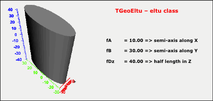
An elliptical tube is defined by the two semi-axes A and B. It ranges from -dZ to +dZ as all other tubes:
A hyperboloid is represented as a solid limited by two planes perpendicular to the Z axis (top and bottom planes) and two hyperbolic surfaces of revolution about Z axis (inner and outer surfaces). The class describing hyperboloids is TGeoHype has 5 input parameters:
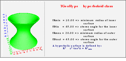
The hyperbolic surface equation is taken in the form:
r,z: cylindrical coordinates for a point on the surface: stereo angle between the hyperbola asymptotic lines and Z axisr2min: minimum distance between hyperbola and Z axis (at z=0)The input parameters represent:
rin, stin: minimum radius and tangent of stereo angle for inner surfacerout, stout: minimum radius and tangent of stereo angle for outer surfacedz: half length in Z (bounding planes positions at +/-dz)The following conditions are mandatory in order to avoid intersections between the inner and outer hyperbolic surfaces in the range +/-dz:
rin<routrout>0rin2 + dz2*stin2 > rout2 + dz2*stout2Particular cases:
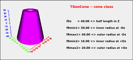
rin=0, stin0: the inner surface is conicalstin=0 / stout=0: cylindrical surface(s)The cones are defined by 5 parameters:
rmin1: internal radius at Z is -dzrmax1: external radius at Z is -dzrmin2: internal radius at Z is +dzrmax2: external radius at Z is +dzdz: half length in Z (a cone ranges from -dz to +dz)A cone has Z-axis as its symmetry axis.
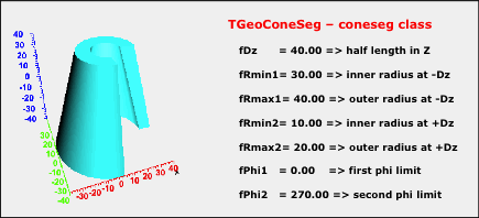
A cone segment is a cone having a range in phi. The cone segment class derives from TGeoCone, having two extra parameters: phi1 and phi2.
TGeoConeSeg(Double_t dz,Double_t rmin1,Double_t rmax1,
Double_t rmin2,Double_t rmax2,Double_t phi1,Double_t phi2);Parametersphi1 and phi2 have the same meaning and convention as for tube segments.
Spheres in TGeo are not just balls having internal and external radii, but sectors of a sphere having defined theta and phi ranges. The TGeoSphere class has the following constructor.
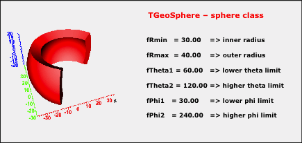
TGeoSphere(Double_t rmin,Double_t rmax,Double_t theta1,
Double_t theta2,Double_t phi1, Double_t phi2);
rmin: internal radius of the spherical sectorrmax: external radiustheta1: starting theta value [0, 180) in degreestheta2: ending theta value (0, 180] in degrees (theta1<theta2)The torus is defined by its axial radius, its inner and outer radius.
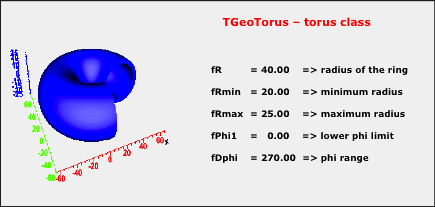
It may have a phirange:
R: axial radius of the torusRmin: inner radiusRmax: outer radiusPhi1: starting phi angleDphi: total phi rangeA paraboloid is defined by the revolution surface generated by a parabola and is bounded by two planes perpendicular to Z axis. The parabola equation is taken in the form: z = a·r2 + b, where: r2 = x2 + y2. Note the missing linear term (parabola symmetric with respect to Z axis).
The coefficients a and b are computed from the input values which are the radii of the circular sections cut by the planes at +/-dz:
-dz = a*r2low + bdz = a*r2high + b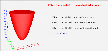
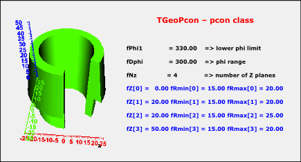
A polycone is represented by a sequence of tubes/cones, glued together at defined Z planes. The polycone might have a phi segmentation, which globally applies to all the pieces. It has to be defined in two steps:
TGeoPcon constructor to define a polycone:phi1: starting phi angle in degreesdphi: total phi rangenz: number of Z planes defining polycone sections (minimum 2)i: section index [0, nz-1]z: z coordinate of the sectionrmin: minimum radius corresponding too this sectionrmax: maximum radius.The first section (i=0) has to be positioned always the lowest Z coordinate. It defines the radii of the first cone/tube segment at its lower Z. The next section defines the end-cap of the first segment, but it can represent also the beginning of the next one. Any discontinuity in the radius has to be represented by a section defined at the same Z coordinate as the previous one. The Z coordinates of all sections must be sorted in increasing order. Any radius or Z coordinate of a given plane have corresponding getters:
Double_t TGeoPcon::GetRmin(Int_t i);
Double_t TGeoPcon::GetRmax(Int_t i);
Double_t TGeoPcon::GetZ(Int_t i);
Note that the last section should be defined last, since it triggers the computation of the bounding box of the polycone.
Polygons are defined in the same way as polycones, the difference being just that the segments between consecutive Z planes are regular polygons. The phi segmentation is preserved and the shape is defined in a similar manner, just that rmin and rmax represent the radii of the circles inscribed in the inner/outer polygon.
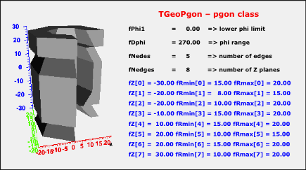
The constructor of a polygon has the form:
The extra parameter nedges represent the number of equal edges of the polygons, between phi1 and phi1+dphi.
A TGeoXtru shape is represented by the extrusion of an arbitrary polygon with fixed outline between several Z sections. Each Z section is a scaled version of the same “blueprint” polygon. Different global XY translations are allowed from section to section. Corresponding polygon vertices from consecutive sections are connected.
An extruded polygon can be created using the constructor:
nplanes:number of Z sections (minimum 2)
The lists of X and Y positions for all vertices have to be provided for the “blueprint” polygon:
nvertices:number of vertices of the polygonxv,yv:arrays of X and Y coordinates for polygon verticesThe method creates an object of the class TGeoPolygon for which the convexity is automatically determined . The polygon is decomposed into convex polygons if needed.
Next step is to define the Z positions for each section plane as well as the XY offset and scaling for the corresponding polygons.
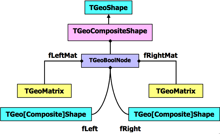
snum:Z section index (0, nplanes-1). The section with snum = nplanes-1 must be defined last and triggers the computation of the bounding box for the whole shapezsection:Z position of section snum. Sections must be defined in increasing order of Z (e.g. snum=0 correspond to the minimum Z and snum=nplanes-1 to the maximum one).x0,y0:offset of section snum with respect to the local shape reference frame Tscale:factor that multiplies the X/Y coordinates of each vertex of the polygon at section snum:x[ivert] = x0 + scale*xv[ivert]y[ivert] = y0 + scale*yv[ivert]Composite shapes are Boolean combinations of two or more shape components. The supported Boolean operations are union (+), intersection (*) and subtraction(-). Composite shapes derive from the base TGeoShape class, therefore providing all shape features: computation of bounding box, finding if a given point is inside or outside the combination, as well as computing the distance to entering/exiting. They can be directly used for creating volumes or used in the definition of other composite shapes.
Composite shapes are provided in order to complement and extend the set of basic shape primitives. They have a binary tree internal structure, therefore all shape-related geometry queries are signals propagated from top level down to the final leaves, while the provided answers are assembled and interpreted back at top. This CSG (composite solid geometry) hierarchy is effective for small number of components, while performance drops dramatically for large structures. Building a complete geometry in this style is virtually possible but highly not recommended.
A composite shape can always be looked as the result of a Boolean operation between only two shape components. All information identifying these two components as well as their positions with respect to the frame of the composite is represented by an object called Boolean node. A composite shape has a pointer to such a Boolean node. Since the shape components may also be composites, they will also contain binary Boolean nodes branching out other two shapes in the hierarchy. Any such branch ends-up when the final leaves are no longer composite shapes, but basic primitives. The figure shows the composite shapes structure.
Suppose that A, B, C and D represent basic shapes, we will illustrate how the internal representation of few combinations look like. We do this only for understanding how to create them in a proper way, since the user interface for this purpose is in fact very simple. We will ignore for the time being the positioning of components. The definition of a composite shape takes an expression where the identifiers are shape names. The expression is parsed and decomposed in 2 sub-expressions and the top-level Boolean operator.
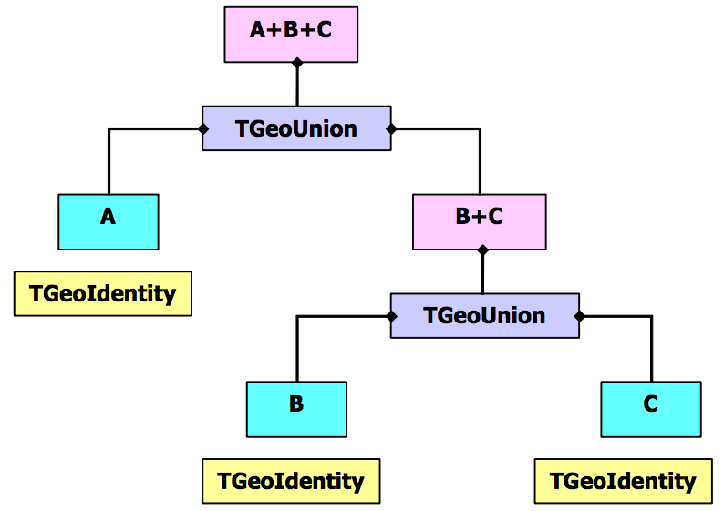
A+B+CJust to illustrate the Boolean expression parsing and the composite shape structure, let’s take a simple example. We will describe the union of A, B and C. Both union operators are at the same level. Since:
A+B+C = (A+B)+C = A+(B+C)
The first(+) is taken as separator, hence the expression split in: A and (B+C). A Boolean node of type TGeoUnion("A","B+C") is created. This tries to replace the 2 expressions by actual pointers to corresponding shapes. The first expression (A) contains no operators therefore is interpreted as representing a shape. The shape named “A” is searched into the list of shapes handled by the manager class and stored as the “left” shape in the Boolean union node. Since the second expression is not yet fully decomposed, the “right” shape in the combination is created as a new composite shape. This will split at its turn B+C into B and C and create a TGeoUnion("B","C"). The B and C identifiers will be looked for and replaced by the pointers to the actual shapes into the new node. Finally, the composite “A+B+C” will be represented as shown in Fig.17-23.**
To build this composite shape:
Any shape entering a Boolean combination can be prior positioned. In order to do so, one has to attach a matrix name to the shape name by using a colon (:). As for shapes, the named matrix has to be prior defined:
TGeoMatrix *mat;
// ... code creating some geometrical transformation
mat->SetName("mat1");
mat->RegisterYourself();  // see Geometrical transformations
An identifier shape:matrix have the meaning: shape is translated or rotated with matrix with respect to the Boolean combination it enters as operand. Note that in the expression A+B+C no matrix identifier was provided, therefore the identity matrix was used for positioning the shape components. The next example will illustrate a more complex case.
(A:m1+B):m2-(C:m3*D:m4):m5Let’s try to understand the expression above. This expression means: subtract the intersection of C and D from the union of A and B. The usage of parenthesis to force the desired precedence is always recommended. One can see that not only the primitive shapes have some geometrical transformations, but also their intermediate compositions.
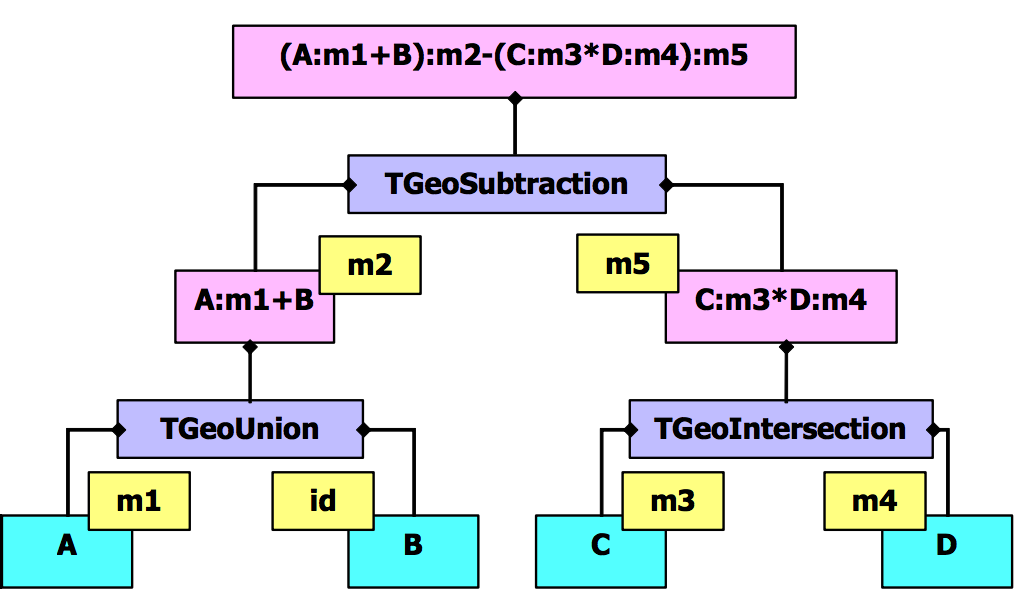
Building composite shapes as in the first example is not always quite useful since we were using un-positioned shapes. When supplying just shape names as identifiers, the created Boolean nodes will assume that the shapes are positioned with an identity transformation with respect to the frame of the created composite. In order to provide some positioning of the combination components, we have to attach after each shape identifier the name of an existing transformation, separated by a colon. Obviously all transformations created for this purpose have to be objects with unique names in order to be properly substituted during parsing.
One should have in mind that the same shape or matrix identifiers can be used many times in the same expression, as in the following example:
const Double_t sq2 = TMath::Sqrt(2.);
gSystem->Load("libGeom");
TGeoManager *mgr =
   new TGeoManager("Geom","composite shape example");
TGeoMedium *medium = 0;
TGeoVolume *top = mgr->MakeBox("TOP",medium,100,250,250);
mgr->SetTopVolume(top);

// make shape components
TGeoBBox *sbox  = new TGeoBBox("B",100,125*sq2,125*sq2);
TGeoTube *stub  = new TGeoTube("T",0,100,250);
TGeoPgon *spgon = new TGeoPgon("P",0.,360.,6,2);
spgon->DefineSection(0,-250,0,80);
spgon->DefineSection(1,250,0,80);

// define some rotations
TGeoRotation *r1 = new TGeoRotation("r1",90,0,0,180,90,90);
r1->RegisterYourself();
TGeoRotation *r2 = new TGeoRotation("r2",90,0,45,90,45,270);
r2->RegisterYourself();
// create a composite
TGeoCompositeShape *cs = new TGeoCompositeShape("cs",
"((T+T:r1)-(P+P:r1))*B:r2");
TGeoVolume *comp = new TGeoVolume("COMP",cs);
comp->SetLineColor(5);

// put it in the top volume
top->AddNode(comp,1);
mgr->CloseGeometry();
// visualize it with ray tracing
top->Raytrace();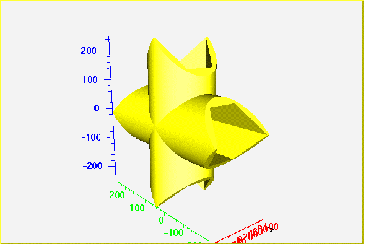
Composite shapes can be subsequently used for defining volumes. Moreover, these volumes contain other volumes, following the general criteria. Volumes created based on composite shapes cannot be divided.
Shapes are named objects and register themselves to the manager class at creation time. This is responsible for their final deletion. Shapes can be created without name if their retrieval by name is no needed. Generally shapes are objects that are useful only at geometry creation stage. The pointer to a shape is in fact needed only when referring to a given volume and it is always accessible at that level. Several volumes may reference a single shape; therefore its deletion is not possible once volumes were defined based on it.
The navigation features related for instance to tracking particles are performed in the following way: Each shape implement its specific algorithms for all required tasks in its local reference system. Note that the manager class handles global queries related to geometry. However, shape-related queries might be sometimes useful:
The method above returns kTRUE if the point *point is actually inside the shape. The point has to be defined in the local shape reference. For instance, for a box having DX,DY and DZhalf-lengths a point will be considered inside if:
-DX <= point[0] <= DX
-DY <= point[1] <= DY
-DZ <= point[2] <= DZ
Double_t TGeoShape::DistFromInside(Double_t *point[3],
Double_t *dir[3], Int_t iact,Double_t step,Double_t *safe);
The method computes the distance to exiting a shape from a given point inside, along a given direction. This direction is given by its director cosines with respect to the local shape coordinate system. This method provides additional information according the value of iact input parameter:
iact = 0computes only safe distance and fill it at the location given by SAFE;iact = 1a proposed STEP is supplied. The safe distance is computed first. If this is bigger than STEP than the proposed step is approved and returned by the method since it does not cross the shape boundaries. Otherwise, the distance to exiting the shape is computed and returned;iact = 2computes both safe distance and distance to exiting, ignoring the proposed step;iact > 2computes only the distance to exiting, ignoring anything elseDouble_t TGeoShape::DistFromOutside(Double_t *point[3],
Double_t *dir[3],Int_t iact,Double_t step,Double_t *safe);This method computes the distance to entering a shape from a given point outside. It acts in the same way as the previous method.
This computes the maximum shift of a point in any direction that does not change its inside/outsidestate (does not cross shape boundaries). The state of the point has to be properly supplied.
The method above computes the director cosines of normal to the crossed shape surface from a given point towards direction. This is filled into the norm array, supplied by the user. The normal vector is always chosen such that its dot product with the direction is positive defined.
Shape objects embeds only the minimum set of parameters that are fully describing a valid physical shape. For instance, the half-length, the minimum and maximum radius represent a tube. Shapes are used together with media in order to create volumes, which in their turn are the main components of the geometrical tree. A specific shape can be created stand-alone:
TGeoBBox *box = new TGeoBBox("s_box",halfX,halfY,halfZ); // named
TGeoTube *tub = new TGeoTube(rmin,rmax,halfZ); // no name
//...  (See all specific shape constructors)
Sometimes it is much easier to create a volume having a given shape in one step, since shapes are not directly linked in the geometrical tree but volumes are:
TGeoVolume *vol_box = gGeoManager->MakeBox("BOX_VOL",pmed,halfX,
halfY,halfZ);
TGeoVolume *vol_tub = gGeoManager->MakeTube("TUB_VOL",pmed,rmin,
rmax,halfZ);
// ...(See MakeXXX() utilities in TGeoManager class)Shapes can generally be divided along a given axis. Supported axes are: X, Y, Z, Rxy, Phi, Rxyz. A given shape cannot be divided however on any axis. The general rule is that that divisions are possible on whatever axis that produces still known shapes as slices. The division of shapes are performed by the call TGeoShape::Divide(), but this operation can be done only via TGeoVolume::Divide() method. In other words, the algorithm for dividing a specific shape is known by the shape object, but is always invoked in a generic way from the volume level. Details on how to do that can be found in the paragraph ‘Dividing volumes’. One can see how all division options are interpreted and which their result inside specific shape classes is.
Shapes generally have a set of parameters that is well defined at build time. In fact, when the final geometrical hierarchy is assembled and the geometry is closed, all constituent shapes MUST**have well defined and valid parameters. In order to ease-up geometry creation, some parameterizations are however allowed.
For instance let’s suppose that we need to define several volumes having exactly the same properties but different sizes. A way to do this would be to create as many different volumes and shapes. The modeller allows however the definition of a single volume having undefined shape parameters.
name: the name of the newly created volume;shape:the type of the associated shape. This has to contain the case-insensitive first 4 letters of the corresponding class name (e.g. “tubs” will match TGeoTubeSeg, “bbox” will match TGeoBBox)nmed: the medium number.This will create a special volume that will not be directly used in the geometry, but whenever positioned will require a list of actual parameters for the current shape that will be created in this process. Such volumes having shape parameters known only when used have to be positioned only with TGeoManager::Node() method (see ‘Creating and Positioning Volumes’).
Other case when shape parameterizations are quite useful is scaling geometry structures. Imagine that we would like to enlarge/shrink a detector structure on one or more axes. This happens quite often in real life and is handled by “fitting mother” parameters. This is accomplished by defining shapes with one or more invalid (negative) parameters. For instance, defining a box having dx=10., dy=10., and dz=-1 will not generate an error but will be interpreted in a different way: A special volume TGeoVolumeMulti will be created. Whenever positioned inside a mother volume, this will create a normal TGeoVolume object having as shape a box with dz fitting the corresponding dzof the mother shape. Generally, this type of parameterization is used when positioning volumes in containers having a matching shape, but it works also for most reasonable combinations.
A given geometry can be built in various ways, but one has to follow some mandatory steps. Even if we might use some terms that will be explained later, here are few general rules:
There is also a list of specific rules:
TGeoManager::CloseGeometry()). Voxelization can be redone per volume after this process.The list is much bigger and we will describe in more detail the geometry creation procedure in the following sections. Provided that geometry was successfully built and closed, the TGeoManager class will register itself to ROOT and the logical/physical structures will become immediately browsable.
The basic components used for building the logical hierarchy of the geometry are the positioned volumes called nodes. Volumes are fully defined geometrical objects having a given shape and medium and possibly containing a list of nodes. Nodes represent just positioned instances of volumes inside a container volume but users do not directly create them. They are automatically created as a result of adding one volume inside other or dividing a volume. The geometrical transformation held by nodes is always defined with respect to their mother (relative positioning). Reflection matrices are allowed.
A hierarchical element is not fully defined by a node since nodes are not directly linked to each other, but through volumes (a node points to a volume, which at its turn points to a list of nodes):
NodeTop VolTop NodeA VolA ...
One can therefore talk about “the node or volume hierarchy”, but in fact, an element is made by a pair volume-node. In the line above is represented just a single branch, but of course from any volume other branches can also emerge. The index of a node in such a branch (counting only nodes) is called depth. The top node have always depth=0.
Volumes need to have their daughter nodes defined when the geometry is closed. They will build additional structures (called voxels ) in order to fasten-up the search algorithms. Finally, nodes can be regarded as bi-directional links between containers and contained volumes.
The structure defined in this way is a graph structure since volumes are replicable (same volume can become daughter node of several other volumes), every volume becoming a branch in this graph. Any volume in the logical graph can become the actual top volume at run time (see TGeoManager::SetTopVolume()). All functionalities of the modeller will behave in this case as if only the corresponding branch starting from this volume is the active geometry.
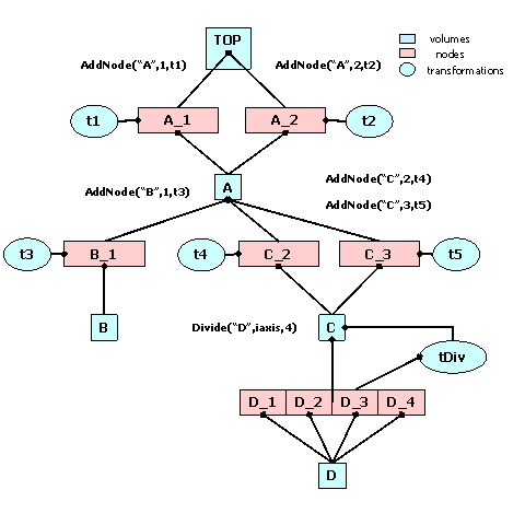
Nodes are never instantiated directly by users, but created as a result of volume operations. Adding a volume named A with a given user id inside a volume B will create a node named A_id. This will be added to the list of nodes stored by B. In addition, when applying a division operation in N slices to a volume A, a list of nodes B_1, B_2, … , B_N is also created. A node B_i does not represent a unique object in the geometry because its container A might be at its turn positioned as node inside several other volumes. Only when a complete branch of nodes is fully defined up to the top node in the geometry, a given path:/TOP_1/…/A_3/B_7 will represent a unique object. Its global transformation matrix can be computed as the pile-up of all local transformations in its branch. We will therefore call logical graph the hierarchy defined by nodes and volumes. The expansion of the logical graph by all possible paths defines a tree structure where all nodes are unique “touchable” objects. We will call this the “physical tree”. Unlike the logical graph, the physical tree can become a huge structure with several millions of nodes in case of complex geometries; therefore, it is not always a good idea to keep it transient in memory. Since the logical and physical structures are correlated, the modeller rather keeps track only of the current branch, updating the current global matrix at each change of the level in geometry. The current physical node is not an object that can be asked for at a given moment, but rather represented by the combination: current node/current global matrix. However, physical nodes have unique ID’s that can be retrieved for a given modeller state. These can be fed back to the modeller in order to force a physical node to become current. The advantage of this comes from the fact that all navigation queries check first the current node; therefore the location of a point in the geometry can be saved as a starting state for later use.
Nodes can be declared as overlapping in case they do overlap with other nodes inside the same container or extrude this container (see also ‘Checking the Geometry’). Non-overlapping nodes can be created with:
The creation of overlapping nodes can be done with a similar prototype:
When closing the geometry, overlapping nodes perform a check of possible overlaps with their neighbors. These are stored and checked all the time during navigation; therefore, navigation is slower when embedding such nodes into geometry. Nodes have visualization attributes as the volume has. When undefined by users, painting a node on a pad will take the corresponding volume attributes.
As mentioned before, volumes are the basic objects used in building the geometrical hierarchy. They represent objects that are not positioned, but store all information about the placement of the other volumes they may contain. Therefore a volume can be replicated several times in the geometry. As it was explained, in order to create a volume, one has to put together a shape and a medium, which are already defined.
Volumes have to be named by users at creation time. Every different name may represent a unique volume object, but may also represent more general a family (class) of volume objects having the same shape type and medium, but possibly different shape parameters. It is the user’s task to provide different names for different volume families in order to avoid ambiguities at tracking time.
A generic family rather than a single volume is created only in two cases: when a parametric shape is used or when a division operation is applied. Each volume in the geometry stores a unique ID corresponding to its family. In order to ease-up their creation, the manager class is providing an API that allows making a shape and a volume in a single step.
// Making a volume out of a shape and a medium.
TGeoVolume *vol = new TGeoVolume("VNAME",ptrShape,ptrMed);

// Making a volume out of a shape but without a defined medium.
TGeoVolume *vol = new TGeoVolume("VNAME",ptrShape);

// Making a volume with a given shape in one step
TGeoVolume *vol = gGeoManager->MakeBox("VNAME",ptrMed,dx,dy,dz);
TGeoVolume *vol = gGeoManager->MakeTubs("VNAME",ptrMed,rmin,rmax,
dz,phi1,phi2);

// See class TGeoManager for the rest of shapes.
// Making a volume with a given shape with a unique prototype
TGeoVolume *vol = gGeoManager->Volume("VNAME","XXXX",nmed,upar,
npar);

// Where XXXX stands for the first 4 letters of the specific shape
// classes, nmed is the medium number, upar is an Double_t * array
// of the shape parameters and npar is the number of parameters.
// This prototype allows (npar = 0) to define volumes with shape
// defined only at positioning time (volumes defined in this way
// need to be positioned using TGeoManager::Node() method)Geometrical modeling is a difficult task when the number of different geometrical objects is 106-108. This is more or less the case for detector geometries of complex experiments, where a ‘flat’ CSG model description cannot scale with the current CPU performances. This is the reason why models like GEANT [1] introduced an additional dimension (depth) in order to reduce the complexity of the problem. This concept is also preserved by the ROOT modeller and introduces a pure geometrical constraint between objects (volumes in our case) - containment. This means in fact that any positioned volume has to be contained by another. Now what means contained and positioned?
contains a point if this is inside the shape associated to the volume. For instance, a volume having a box shape will contain all points P=(X,Y,Z) verifying the conditions: Abs(Pi)dXi. The points on the shape boundaries are considered as inside the volume. The volume contains a daughter if it contains all the points contained by the daughter.Positioning a volume inside another have to introduce a geometrical transformation between the two. If M defines this transformation, any point in the daughter reference can be converted to the mother reference by: Pmother = MPdaughterWhen creating a volume one does not specify if this will contain or not other volumes. Adding daughters to a volume implies creating those and adding them one by one to the list of daughters. Since the volume has to know the position of all its daughters, we will have to supply at the same time a geometrical transformation with respect to its local reference frame for each of them.
The objects referencing a volume and a transformation are called NODES and their creation is fully handled by the modeller. They represent the link elements in the hierarchy of volumes. Nodes are unique and distinct geometrical objects ONLY from their container point of view. Since volumes can be replicated in the geometry, the same node may be found on different branches.
In order to provide navigation features, volumes have to be able to find the proper container of any point defined in the local reference frame. This can be the volume itself, one of its positioned daughter volumes or none if the point is actually outside. On the other hand, volumes have to provide also other navigation methods such as finding the distances to its shape boundaries or which daughter will be crossed first. The implementation of these features is done at shape level, but the local mother-daughters management is handled by volumes. These build additional optimization structures upon geometry closure. In order to have navigation features properly working one has to follow some rules for building a valid geometry.
The daughter nodes of a volume can be also removed or replaced with other nodes:
void RemoveNode(TGeoNode* node)
TGeoNode*ReplaceNode(TGeoNode* nodeorig, TGeoShape* newshape = 0,
TGeoMatrix* newpos = 0, TGeoMedium* newmed = 0)
The last method allows replacing an existing daughter of a volume with another one. Providing only the node to be replaced will just create a new volume for the node but having exactly the same parameters as the old one. This helps in case of divisions for decoupling a node from the logical hierarchy so getting new content/properties. For non-divided volumes, one can change the shape and/or the position of the daughter.
Virtual containers are volumes that do not represent real objects, but they are needed for grouping and positioning together other volumes. Such grouping helps not only geometry creation, but also optimizes tracking performance; therefore, it is highly recommended. Virtual volumes need to inherit material/medium properties from the volume they are placed into in order to be “invisible” at tracking time.
Let us suppose that we need to group together two volumes A and B into a structure and position this into several other volumes D,E, and F. What we need to do is to create a virtual container volume C holding A and B, then position C in the other volumes.
Note that C is a volume having a determined medium. Since it is not a real volume, we need to manually set its medium the same as that of D,E or F in order to make it ‘invisible’ (same physics properties). In other words, the limitation in proceeding this way is that D,E, and F must point to the same medium. If this was not the case, we would have to define different virtual volumes for each placement: C, C' and C", having the same shape but different media matching the corresponding containers. This might not happen so often, but when it does, it forces the creation of several extra virtual volumes. Other limitation comes from the fact that any container is directly used by navigation algorithms to optimize tracking. These must geometrically contain their belongings (positioned volumes) so that these do not extrude its shape boundaries. Not respecting this rule generally leads to unpredictable results. Therefore A and B together must fit into C that has to fit also into D,E, and F. This is not always straightforward to accomplish, especially when instead of A and B we have many more volumes.
In order to avoid these problems, one can use for the difficult cases the class TGeoVolumeAssembly, representing an assembly of volumes. This behaves like a normal container volume supporting other volumes positioned inside, but it has neither shape nor medium. It cannot be used directly as a piece of the geometry, but just as a temporary structure helping temporary assembling and positioning volumes.
If we define now C as an assembly containing A and B, positioning the assembly into D,E and F will actually position only A and Bdirectly into these volumes, taking into account their combined transformations A/B to C and C to D/E/F. This looks much nicer, is it? In fact, it is and it is not. Of course, we managed to get rid of the ‘unnecessary’ volume C in our geometry, but we end-up with a more flat structure for D,E and F (more daughters inside). This can get much worse when extensively used, as in the case: assemblies of assemblies.
For deciding what to choose between using virtual containers or assemblies for a specific case, one can use for both cases, after the geometry was closed:
The ptr_D is a pointer to volume D containing the interesting structure. The test will provide the timing for classifying 1 million random points inside D.
Now let us make a simple volume representing a copper wire. We suppose that a medium is already created (see TGeoMedium class on how to create media).
We will create a TUBE shape for our wire, having Rmin=0cm, Rmax=0.01cm and a half-length dZ=1cm:
One may omit the name for the shape wire_tube, if no retrieving by name is further needed during geometry building. Different volumes having different names and materials can share the same shape.
Now let’s make the volume for our wire:
(*) Do not bother to delete the media, shapes or volumes that you have created since all will be automatically cleaned on exit by the manager class.
If we would have taken a look inside TGeoManager::MakeTube() method, we would have been able to create our wire with a single line:
(*) The same applies for all primitive shapes, for which there can be found corresponding MakeSHAPE() methods. Their usage is much more convenient unless a shape has to be shared between more volumes.
Let us make now an aluminum wire having the same shape, supposing that we have created the copper wire with the line above:
We would like now to position our wire in the middle of a gas chamber. We need first to define the gas chamber:
Now we can put the wire inside:
If we inspect now the chamber volume in a browser, we will notice that it has one daughter. Of course, the gas has some container also, but let us keeps it like that for the sake of simplicity. Since we did not supply the third argument, the wire will be positioned with an identity transformation inside the chamber.
Positioning volumes that does not overlap their neighbors nor extrude their container is sometimes quite strong constraint. Having a limited set of geometric shapes might force sometimes overlaps. Since overlapping is contradictory to containment, a point belonging to an overlapping region will naturally belong to all overlapping partners. The answer provided by the modeller to “Where am I?” is no longer deterministic if there is no priority assigned.
There are two ways out provided by the modeller in such cases and we will illustrate them by examples.
Rmin=0,Rmax=inner/outer radius), then to make a composite:C = (Tub1out+Tub2out)-(Tub1in+Tub2in)This will instruct the modeller that the daughter ROW inside CAL overlaps with something else. The modeller will check this at closure time and build a list of possibly overlapping candidates. This option is equivalent with the option MANY in GEANT3.
The modeller supports such cases only if user declares the overlapping nodes. In order to do that, one should use TGeoVolume::AddNodeOverlap() instead of TGeoVolume::AddNode(). When two or more positioned volumes are overlapping, not all of them have to be declared so, but at least one. A point inside an overlapping region equally belongs to all overlapping nodes, but the way these are defined can enforce the modeller to give priorities.
The general rule is that the deepest node in the hierarchy containing a point has the highest priority. For the same geometry level, non-overlapping is prioritized over overlapping. In order to illustrate this, we will consider few examples. We will designate non-overlapping nodes as ONLY and the others MANY as in GEANT3, where this concept was introduced:
The part of a MANY node B extruding its container A will never be “seen” during navigation, as if B was in fact the result of the intersection of A and B.
If we have two nodes A (ONLY) and B (MANY) inside the same container, all points in the overlapping region of A and B will be designated as belonging to A.
If A an B in the above case were both MANY, points in the overlapping part will be designated to the one defined first. Both nodes must have the same medium.
The slices of a divided MANY will be as well MANY.
One needs to know that navigation inside geometry parts MANY nodes is much slower. Any overlapping part can be defined based on composite shapes - might be in some cases a better way out.
What can we do if our chamber contains two identical wires instead of one? What if then we would need 1000 chambers in our detector? Should we create 2000 wires and 1000 chamber volumes? No, we will just need to replicate the ones that we have already created.
chamber->AddNode(wire_co,1,new TGeoTranslation(0.2,0,0));
chamber->AddNode(wire_co,2,new TGeoTranslation(0.2,0,0));
The 2 nodes that we have created inside chamber will both point to a wire_co object, but will be completely distinct: WIRE_CO_1 and WIRE_CO_2. We will want now to place symmetrically 1000 chambers on a pad, following a pattern of 20 rows and 50 columns. One way to do this will be to replicate our chamber by positioning it 1000 times in different positions of the pad. Unfortunately, this is far from being the optimal way of doing what we want. Imagine that we would like to find out which of the 1000 chambers is containing a (x,y,z) point defined in the pad reference. You will never have to do that, since the modeller will take care of it for you, but let’s guess what it has to do. The most simple algorithm will just loop over all daughters, convert the point from mother to local reference and check if the current chamber contains the point or not. This might be efficient for pads with few chambers, but definitely not for 1000. Fortunately the modeller is smarter than that and creates for each volume some optimization structures called voxels to minimize the penalty having too many daughters, but if you have 100 pads like this in your geometry you will anyway lose a lot in your tracking performance. The way out when volumes can be arranged according to simple patterns is the usage of divisions. We will describe them in detail later on. Let’s think now at a different situation: instead of 1000 chambers of the same type, we may have several types of chambers. Let’s say all chambers are cylindrical and have a wire inside, but their dimensions are different. However, we would like all to be represented by a single volume family, since they have the same properties.
A volume family is represented by the class TGeoVolumeMulti. It represents a class of volumes having the same shape type and each member will be identified by the same name and volume ID. Any operation applied to a TGeoVolumeMulti equally affects all volumes in that family. The creation of a family is generally not a user task, but can be forced in particular cases:
Where: vname is the family name, nmed is the medium number and shape is the shape type that can be:
boxfor TGeoBBoxtrd1for TGeoTrd1trd2for TGeoTrd2trapfor TGeoTrapgtrafor TGeoGtraparafor TGeoParatube, tubsfor TGeoTube, TGeoTubeSegcone, consfor TGeoCone, TGeoConseltufor TGeoEltuctubfor TGeoCtubpconfor TGeoPconpgonfor TGeoPgonVolumes are then added to a given family upon adding the generic name as node inside other volume:
TGeoVolume *box_family = gGeoManager->Volume("BOXES","box",nmed);
//   ...
gGeoManager->Node("BOXES",Int_t copy_no,"mother_name",Double_t x,
Double_t y,Double_t z,Int_t rot_index,Bool_t is_only,
Double_t *upar,Int_t npar);BOXES- name of the family of boxescopy_no- user node number for the created nodemother_name- name of the volume to which we want to add the nodex,y,z- translation componentsrot_index- index of a rotation matrix in the list of matricesupar- array of actual shape parametersnpar- number of parametersThe parameters order and number are the same as in the corresponding shape constructors. Another particular case where volume families are used is when we want that a volume positioned inside a container to match one ore more container limits. Suppose we want to position the same box inside 2 different volumes and we want the Z size to match the one of each container:
TGeoVolume *container1 = gGeoManager->MakeBox("C1",imed,10,10,30);
TGeoVolume *container2 = gGeoManager->MakeBox("C2",imed,10,10,20);
TGeoVolume *pvol       = gGeoManager->MakeBox("PVOL",jmed,3,3,-1);
container1->AddNode(pvol,1);
container2->AddNode(pvol,1);
Note that the third parameter of PVOL is negative, which does not make sense as half-length on Z. This is interpreted as: when positioned, create a box replacing all invalid parameters with the corresponding dimensions of the container. This is also internally handled by the TGeoVolumeMulti class, which does not need to be instantiated by users.
Volumes can be divided according a pattern. The simplest division can be done along one axis that can be: X,Y,Z,Phi,Rxy or Rxyz. Let’s take a simple case: we would like to divide a box in N equal slices along X coordinate, representing a new volume family. Supposing we already have created the initial box, this can be done like:
Here SLICEX is the name of the new family representing all slices and 1 is the slicing axis. The meaning of the axis index is the following: for all volumes having shapes like box, trd1, trd2, trap, gtraorpara -1, 2, 3 mean X, Y, Z; for tube, tubs, cone, cons -1 means Rxy, 2 means phi and 3 means Z; for pcon and pgon - 2 means phi and 3 means Z; for spheres 1 means Rand 2 means phi.
In fact, the division operation has the same effect as positioning volumes in a given order inside the divided container - the advantage being that the navigation in such a structure is much faster. When a volume is divided, a volume family corresponding to the slices is created. In case all slices can be represented by a single shape, only one volume is added to the family and positioned N times inside the divided volume, otherwise, each slice will be represented by a distinct volume in the family.
Divisions can be also performed in a given range of one axis. For that, one has to specify also the starting coordinate value and the step:
A check is always done on the resulting division range: if not fitting into the container limits, an error message is posted. If we will browse the divided volume we will notice that it will contain N nodes starting with index 1 up to N. The first one has the lower X limit at START position, while the last one will have the upper X limit at START+N*STEP. The resulting slices cannot be positioned inside another volume (they are by default positioned inside the divided one) but can be further divided and may contain other volumes:
When doing that, we have to remember that SLICEY represents a family, therefore all members of the family will be divided on Y and the other volume will be added as node inside all.
In the example above all the resulting slices had the same shape as the divided volume (box). This is not always the case. For instance, dividing a volume with TUBE shape on PHIaxis will create equal slices having TUBESEG shape. Other divisions can also create slices having shapes with different dimensions, e.g. the division of a TRD1 volume on Z.
When positioning volumes inside slices, one can do it using the generic volume family (e.g. slicey). This should be done as if the coordinate system of the generic slice was the same as the one of the divided volume. The generic slice in case of PHI division is centered with respect to X-axis. If the family contains slices of different sizes, any volume positioned inside should fit into the smallest one.
Examples for specific divisions according to shape types can be found inside shape classes.
Create a new volume by dividing an existing one (GEANT3 like).
Divides MOTHER into NDIV divisions called NAME along axis IAXIS starting at coordinate value START and having size STEP. The created volumes will have tracking media ID=NUMED (if NUMED=0 -> same media as MOTHER).
The behavior of the division operation can be triggered using OPTION (case insensitive):
Ndivide all range in NDIV cells (same effect as STEP<=0) (GSDVN in G3)NXdivide range starting with START in NDIV cells (GSDVN2 in G3)Sdivide all range with given STEP; NDIV is computed and divisions will be centered in full range (same effect as NDIV<=0) (GSDVS, GSDVT in G3)SXsame as DVS, but from START position (GSDVS2, GSDVT2 in G3)In general, geometry contains structures of positioned volumes that have to be grouped and handled together, for different possible reasons. One of these is that the structure has to be replicated in several parts of the geometry, or it may simply happen that they really represent a single object, too complex to be described by a primitive shape.
Usually handling structures like these can be easily done by positioning all components in the same container volume, then positioning the container itself. However, there are many practical cases when defining such a container is not straightforward or even possible without generating overlaps with the rest of the geometry. There are few ways out of this:
The first two approaches have the disadvantage of penalizing the navigation performance with a factor increasing more than linear of the number of components in the structure. The best solution is the third one because it uses all volume-related navigation optimizations. The class TGeoVolumeAssembly represents an assembly volume. Its shape is represented by TGeoShapeAssembly class that is the union of all components. It uses volume voxelization to perform navigation tasks.
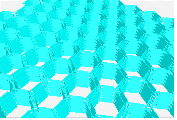
An assembly volume creates a hierarchical level and it geometrically insulates the structure from the rest (as a normal volume). Physically, a point that is INSIDE a TGeoShapeAssembly is always inside one of the components, so a TGeoVolumeAssembly does not need to have a medium. Due to the self-containment of assemblies, they are very practical to use when a container is hard to define due to possible overlaps during positioning. For instance, it is very easy creating honeycomb structures. A very useful example for creating and using assemblies can be found at: http://root.cern.ch/root/html/examples/assembly.C.html.
Creation of an assembly is very easy: one has just to create a TGeoVolumeAssembly object and position the components inside as for any volume:
TGeoVolume *vol = new TGeoVolumeAssembly(name);
vol->AddNode(vdaughter1, cpy1, matrix1);
vol->AddNode(vdaughter2, cpy2, matrix2);
Note that components cannot be declared as “overlapping” and that a component can be an assembly volume. For existing flat volume structures, one can define assemblies to force a hierarchical structure therefore optimizing the performance. Usage of assemblies does NOT imply penalties in performance, but in some cases, it can be observed that it is not as performing as bounding the structure in a container volume with a simple shape. Choosing a normal container is therefore recommended whenever possible.
All geometrical transformations handled by the modeller are provided as a built-in package. This was designed to minimize memory requirements and optimize performance of point/vector master-to-local and local-to-master computation. We need to have in mind that a transformation in TGeo has two major use-cases. The first one is for defining the placement of a volume with respect to its container reference frame. This frame will be called ‘master’ and the frame of the positioned volume - ‘local’. If T is a transformation used for positioning volume daughters, then: MASTER = T * LOCAL
Therefore Tis used to perform a local to master conversion, while T-1 for a master to local conversion. The second use case is the computation of the global transformation of a given object in the geometry. Since the geometry is built as ‘volumes-inside-volumes’, the global transformation represents the pile-up of all local transformations in the corresponding branch. Once a given object in the hierarchy becomes the current one, the conversion from master to local coordinates or the other way around can be done from the manager class.
A general homogenous transformation is defined as a 4x4 matrix embedding a rotation, a translation and a scale. The advantage of this description is that each basic transformation can be represented as a homogenous matrix, composition being performed as simple matrix multiplication.
Rotation: \(\left|\begin{array}{cccc} r_{11} & r_{12} & r_{13} & 0 \\ r_{21} & r_{22} & r_{23} & 0 \\ r_{31} & r_{32} & r_{33} & 0 \\ 0 & 0 & 0 & 1 \end{array} \right|\) Translation: \(\left|\begin{array}{cccc} 1 & 0 & 0 & 0 \\ 0 & 1 & 0 & 0 \\ 0 & 0 & 1 & 0 \\ t_x & t_y & t_z & 1 \end{array} \right|\) Scale: \(\left|\begin{array}{cccc} s_x & 0 & 0 & 0 \\ 0 & s_y & 0 & 0 \\ 0 & 0 & s_z & 0 \\ 0 & 0 & 0 & 1 \end{array} \right|\)
Inverse rotation: \(\left|\begin{array}{cccc} r_{11} & r_{21} & r_{31} & 0 \\ r_{12} & r_{22} & r_{32} & 0 \\ r_{13} & r_{23} & r_{33} & 0 \\ 0 & 0 & 0 & 1 \end{array} \right|\) Inverse translation: \(\left|\begin{array}{cccc} 1 & 0 & 0 & 0 \\ 0 & 1 & 0 & 0 \\ 0 & 0 & 1 & 0 \\ -t_x & -t_y & -t_z & 1 \end{array} \right|\) Inverse scale: \(\left|\begin{array}{cccc} \frac{1}{s_x} & 0 & 0 & 0 \\ 0 & \frac{1}{s_y} & 0 & 0 \\ 0 & 0 & \frac{1}{s_z} & 0 \\ 0 & 0 & 0 & 1 \end{array} \right|\)
The disadvantage in using this approach is that computation for 4x4 matrices is expensive. Even combining two translations would become a multiplication of their corresponding matrices, which is quite an undesired effect. On the other hand, it is not a good idea to store a translation as a block of 16 numbers. We have therefore chosen to implement each basic transformation type as a class deriving from the same basic abstract class and handling its specific data and point/vector transformation algorithms.
The base class TGeoMatrix defines abstract methods for:
TGeoTranslation rotation array through the base TGeoMatrix interface is a legal operation. The answer in this case is a pointer to a global constant array representing an identity rotation.Double_t *TGeoMatrix::GetTranslation() const;
Double_t *TGeoMatrix::GetRotation() const;
Double_t *TGeoMatrix::GetScale() const;void TGeoMatrix::MasterToLocal(const Double_t *master,
Double_t *local)
void TGeoMatrix::LocalToMaster(const Double_t *local,
Double_t *master)
void TGeoMatrix::MasterToLocalVect(const Double_t *master,
Double_t *local)
void TGeoMatrix::LocalToMasterVect(const Double_t *local,
Double_t *master)Here master and local are arrays of size 3. These methods allow correct conversion also for reflections.
Bool_t TGeoMatrix::IsIdentity() const;
Bool_t TGeoMatrix::IsTranslation() const;
Bool_t TGeoMatrix::IsRotation() const;
Bool_t TGeoMatrix::IsScale() const;
Bool_t TGeoMatrix::IsCombi() const;   // (tr. + rot.)
Bool_t TGeoMatrix::IsGeneral() const; // (tr. + rot. + scale)
Specific classes deriving from TGeoMatrix represent combinations of basic transformations. In order to define a matrix as a combination of several others, a special class TGeoHMatrix is provided. Here is an example of matrix creation:
TGeoRotation r1,r2;
r1.SetAngles(90,0,30);          //rotation defined by Euler angles
r2.SetAngles(90,90,90,180,0,0); //rotation defined by GEANT3 angles
TGeoTranslation t1(-10,10,0);
TGeoTranslation t2(10,-10,5);
TGeoCombiTrans c1(t1,r1);
TGeoCombiTrans c2(t2,r2);
TGeoHMatrix h = c1 * c2; // composition is done via TGeoHMatrix
TGeoHMatrix *ph = new TGeoHMatrix(hm); // class it is what we want
                                       // to use for positioning
                                       // a volume
ph->Print();
...
pVolume->AddNode(pVolDaughter,id,ph) // now ph is owned by
the managerUnless explicitly used for positioning nodes (TGeoVolume::AddNode()) all matrices deletion have to be managed by users. Matrices passed to geometry have to be created by using new() operator and TGeoManager class is responsible for their deletion. Matrices that are used for the creation of composite shapes have to be named and registered to the manager class:
Generally, it is advisable to create all intermediate transformations used for making the final combined one on the heap:
TGeoRotation r1(...);
TGeoRotation r2(...);
TGeoHMatrix *mat = new TGeoHMatrix("name"); // we want to use only
                        // this one in geometry
*mat = r1 * r2;TGeoTranslation class) represent a (dx,dy,dz) translation. The only data member is: Double_t fTranslation[3]. Translations can be added or subtracted.TGeoTranslation t1;
t1->SetTranslation(-5,10,4);
TGeoTranslation *t2 = new TGeoTranslation(4,3,10);
t2->Subtract(&t1);TGeoRotation class) represent a pure rotation. Data members are Double_t fRotationMatrix[3*3]. Rotations can be defined either by Euler angles, either, by GEANT3 angles:This represents the composition of: first a rotation about Z axis with angle phi, then a rotation with theta about the rotated X axis, and finally a rotation with psiabout the new Z axis.
This is a rotation defined in GEANT3 style. Theta and phi are the spherical angles of each axis of the rotated coordinate system with respect to the initial one. This construction allows definition of malformed rotations, e.g. not orthogonal. A check is performed and an error message is issued in this case.
Specific utilities: determinant, inverse.
TGeoScale class) - represent a scaled shrinking/enlargement, possibly different on all axes. Data members: Double_t fScale[3]. Not implemented yet.Double_t fTranslation[3],TGeoRotation *fRotation.TGeoRotation *rot = new TGeoRotation("rot",10,20,30);
TGeoTranslation trans;
...
TGeoCombiTrans *c1 = new TGeoCombiTrans(trans,rot);
TGeoCombiTrans *c2 = new TGeoCombiTrans("somename",10,20,30,rot)TGeoHMatrix class) represent combined transformations in any order.TGeoIdentity class) is a generic identity transformation represented by a singleton class object gGeoIdentity.The class TGeoManager class contains the entire API needed for building and tracking geometry. It defines a global pointer gGeoManager in order to be fully accessible from external code. The manager class is the owner of all geometry objects defined in a session; therefore, users must not try to control their deletion. It contains lists of media, materials, transformations, shapes and volumes. A special case is the one of geometrical transformations. When creating a matrix or a translation, this is by default owned by external objects. The manager class becomes owner of all transformations used for positioning volumes. In order to force the ownership for other transformations, one can use TGeoMatrix::RegisterYourself() method. Do not be therefore surprised that some transformations cannot be found by name when creating a composite shape for instance if you did not register them after creation.
Logical nodes (positioned volumes) are created and destroyed by the TGeoVolume class. Physical nodes and their global transformations are subjected to a caching mechanism due to the sometimes very large memory requirements of logical graph expansion. The total number of physical instances of volumes triggers the caching mechanism and the cache manager is a client of TGeoManager. The manager class also controls the drawing/checking package (TGeoPainter client). This is linked with ROOT graphical libraries loaded on demand in order to control visualization actions.
Tracking is the feature allowing the transport of a given particle knowing its kinematics. A state is determined by any combination of the position \(\vec{r}\) and direction \(\vec{n}\) with respect to the world reference frame. The direction \(\vec{n}\) must be a unit vector having as components the director cosines. The full classification of a given state will provide the following information: the deepest physical node containing the position vector, the distance to the closest boundary along the direction vector, the next physical node after propagating the current point with this distance and the safety distance to the nearest boundary. This information allows the propagation of particles inside a detector geometry by taking into account both geometrical and physical constraints.
We will hereby describe the user interface of TGeo to access tracking functionality. This allows either developing a tracker for simple navigation within a given geometry, either interfacing to an external tracking engine such as GEANT. Note that the abstract interface for external trackers can be found in $ROOTSYS/vmc folder and it can be used to run GEANT3, GEANT4 and FLUKA-based simulations (*) by using directly a geometry described with ROOT.
The interface methods related to tracking are incorporated into TGeoManager class and implemented in the navigator class TGeoNavigator. In order to be able to start tracking, one has to define the initial state providing the starting point \(\vec{r_0}\) and direction \(\vec{n_0}\) . There are several ways of doing that.
One geometry may have several independent navigators to query to localize points or compute distances. The geometry manager holds a list of active navigators accessible via:
Upon closing the geometry a default navigator is provided as first one in this list, but one may add its own via:
TGeoNavigator *navig = new TGeoNavigator(gGeoManager);
// Store the index of the user navigator
Int_t inav = gGeoManager->AddNavigator(navig);
// Make its own navigator the active one
gGeoManager->SetCurrentNavigator(inav);
// Switch between navigators
gGeoManager->SetCurrentNavigator(0);
A navigator holds several variables describing the current navigation state: current point position, current direction distance to next boundary, isotropic safety, pointer to current and next nods as well as several tracking flags related to volume boundary conditions or other properties required for track propagation in geometry. Each geometry query affects these variables, so the only way in testing several navigation alternatives and remembering the active navigation state is to use parallel navigation. The following paragraphs will describe the usage of a single navigator. All setters/getters for navigation state parameters as well as navigation queries provided by TGeoNavigator are interfaced by TGeoManager and will act on the current navigator.
The current point (x,y,z) known by the modeller is stored as Double_t fCurrentPoint[3] by the navigator class. This array of the three coordinates is defined in the current global reference system and can be retrieved any time:
Initializing this point can be done like:
In order to move inside geometry starting with the current point, the modeller needs to know the current direction (nx,ny,nz). This direction is stored as Double_t fCurrentDirection[3] by the navigator and it represents a direction in the global frame. It can be retrieved with:
The direction can be initialized in a similar manner as the current point:
Setting the initial point and direction is not enough for initializing tracking. The modeller needs to find out where the initial point is located in the geometrical hierarchy. Due to the containment based architecture of the model, this is the deepest positioned object containing the point. For illustrating this, imagine that we have a simple structure with a top volume A and another one Bpositioned inside. Since Ais a top volume, its associated node A_1 will define MARS and our simple hierarchy of nodes (positioned volumes) will be: /A_1/B_1. Suppose now that the initial point is contained by B_1. This implies by default that the point is also contained by A_1, since B_1 have to be fully contained by this. After searching the point location, the modeller will consider that the point is located inside B_1, which will be considered as the representative object (node) for the current state. This is stored as: TGeoNode *TGeoManager::fCurrentNodeand can be asked from the manager class only after the 'Where am I?' was completed:
In order to find the location of the current point inside the hierarchy of nodes, after setting this point it is mandatory to call the ‘Where am I?' method:
In order to have more flexibility, there are in fact several alternative ways of initializing a modeller state:
// Setting the point and finding the state in one step:
gGeoManager->FindNode(Double_t x,Double_t y,Double_t z);
gGeoManager->FindNode(Double_t *point[3]);
// Setting both initial point and direction and finding the state:
gGeoManager->InitTrack(Double_t x,Double_t y,Double_t z,
Double_t nx, Double_t ny, Double_t nz);
gGeoManager->InitTrack(Double_t *point[3],Double_t *dir[3]);
Note that the current point coordinates can be changed and the state re-initialized at any time. This represents the ‘Where am I?' geometrical query representing the basic navigation functionality provided by the modeller.
The current state and all variables related to this are essential during tracking and have to be checked several times. Besides the current point and direction, the following additional information can be retrieved from TGeoManager interface:
current path. This represents a string containing the names and copy numbers of all positioned objects in the current branch written in the /folder/folder/…/folder/file fashion. The final node pointed by the path is the deepest object containing the current point and is representative for the current state. All intermediate folders in the path are in fact also nodes “touched” by the current point, but having some “touched” containment. The current path can be retrieved only after the state was initialized and is useful for getting an idea of the current point location.const char *path = gGeoManager->GetPath();
cout << "Current path is: " << path << endl;
/A_1/B_34/C_3/D_1current node,volume and material. In order to take decisions on post-step or further stepping actions, one has to know these. In order to get a pointer to the current node one can do:TGeoNode *cnode = gGeoManager->GetCurrentNode();
// then:
TGeoVolume *cvol = gGeoManager->GetCurrentVolume();
// or:
cvol = cnode->GetVolume(); // (*)
// then:
TGeoMaterial *cmat = cvol->GetMedium()->GetMaterial();(*) Note: If the current point is in fact outside the geometry, the current node pointer will not be NULL, but pointing to the top node.
In order to take decisions in such case one needs always to test:
Specific information related to the current volume/node like ID’s or shape can be then retrieved from the corresponding objects.
index. The number of possible different states of the modeller corresponds to the number of different objects/paths in the geometry. This has nothing to do with the number of nodes, since the same node can be found on different branches. In other words, the number of states corresponds to the number of nodes in the expanded geometry tree. Since unfortunately this expansion from logical to physical hierarchy cannot be stored on regular basis due to the large size of the latter, one cannot directly assign state numbers. If the size of the expansion proves however to be small enough (less than about 50 million objects), a parallel structure storing these state indices is built and stored in memory. In such case each state automatically gets an index that can be retrieved after any state initialization. These indices can prove to be quite useful for being able to keep track of the navigation history and force certain states. Let’s illustrate how this works with a simple example:T_1, A_1, A_2, B_1, B_2. On the other hand we will have more states than logical nodes:/T_1- 1 state at level = 0/T_1/A_1,/T_1/A_2- 2 states at level = 1/T_1/A_1/B_1,/T_1/A_1/B_2,/T_1/A_2/B_1,/T_1/A_2/B_2 - 4 states at level = 2gGeoManager->InitTrack(pt,dir); // anything to initialize a state
Int_t istate = gGeoManager->GetCurrentNodeId(); // in fact state Id
{
//... code changing the current state
}
gGeoManager->CdNode(istate); // forces state's re-initializationglobal transformation. This represents the transformation from MARS to the local reference of the current node, being the product of all local mother-daughter transformations in the branch. The global transformation can be referenced or copied:const TGeoHMatrix *global = gGeoManager->GetCurrentMatrix();
TGeoHMatrix *copy = new TGeoHMatrix(*global);master-to-local and local-to-master point and vector conversions to get from MARS to the local node coordinates. This can be done by using the global transformation or directly the TGeoManager corresponding interfaces:Double_t *glob_pt = gGeoManager->GetCurrentPoint();
Double_t *glob_dir = gGeoManager->GetCurrentDirection();
Double_t loc_pt[3], loc_dir[3];
// Go from MARS to local coordinates:
gGeoManager->MasterToLocal(glob_pt,loc_pt); // or:
global->MasterToLocal(glob_pt,loc_pt); // will be omitted from nowAs we already described, saving and restoring modeller states can be quite useful during tracking and is a feature extensively used by external tracking engines. We will call this navigation history management, which in most of the cases can be performed by handling the state identifiers. For quite big geometries, state indexing is not possible anymore and will be automatically disabled by the modeller. Fortunately there is a backup solution working in any condition: the modeller maintains a stack of states that is internally used by its own navigation algorithms, but user code is also allowed to access it. This works on any stack principle by using PUSH and POP calls and user code is responsible for popping the pushed states in order to keep the stack clean.
// push the current state in the stack
Int_t index = gGeoManager->PushPath();
// push state and current point
Int_t index = gGeoManager->PushPoint();
// retrieves the last pushed state (decrements stack index)
gGeoManager->PopPath();
// the same but retrieves also the point location
gGeoManager->PopPoint();
// just decrement stack index without changing state
gGeoManager->PopDummy();
// retrieves a state at given index without changing stack index
gGeoManager->PopPath(Int_t index);After initializing the current state related to a given point and direction defined in MARS (‘Where am I?'), one can query for several geometrical quantities. All the related algorithms work in the assumption that the current point has been localized inside the geometry (by the methods TGeoManager::FindNode() or TGeoManager::InitTrack()) and the current node or path has not been changed by the user.
One can find fast if a point different from the current one has or not the same location inside the geometry tree. To do that, the new point should not be introduced by using TGeoManager::SetCurrentPoint() method, but rather by calling the specific method:
In the prototype above, x, y and z are the coordinates of the new point. The modeller will check whether the current volume still contains the new point or its location has changed in the geometry hierarchy. If the new location is different, two actions are possible according to the value of change:
change = kFALSE (default) - the modeller does not change the current state but just inform the caller about this change.change = kTRUE - the modeller will actually perform a new ‘Where am I?'search after finding out that the location has changed. The current state will be actualized accordingly.Note that even when performing a normal search on the current state after changing the current point coordinates (e.g. gGeoManager->FindNode(newX,newY,newZ)), users can always query if the previous state has changed by using a method having the same name but without parameters:
All tracking engines need to compare the currently proposed physical step with the maximum allowed distance in the current material. The modeller provides this information by computing the distance to the first boundary starting from the current point along a straight line. The starting point and direction for this procedure are the ones corresponding to the current state. The boundary search is initialized inside the current volume and the crossed boundary can belong either to the current node or to one of its daughters. The full prototype of the method is:
In the prototype above, besides the current point and direction that are supposed already initialized, the only input parameter is step. This represents the maximum step allowed by the tracking algorithm or the physical step. The modeller will search for a boundary crossing only up to a distance equal to this value. If a boundary is found, a pointer to the object (node) having it is returned; otherwise the method returns NULL.
The computed value for the computed distance can be subsequently retrieved from the manager class:
According the step value, two use cases are possible:
step = TGeoShape::kBig(default behavior; kBig = 1030). In this case, there is no limitation on the search algorithm, the first crossed node is returned and the corresponding distance computed. If the current point is outside geometry and the top node is not crossed, the corresponding distance will be set to kBig and a NULL pointer returned. No additional quantity will be computed.step < kBig. In this case, the progressive search starting from the current point will be stopped after a distance equal with the supplied step. In addition to the distance to the first crossed boundary, the safety radius is also computed. Whenever the information regarding the maximum required step is known it is recommended to be provided as input parameter in order to speed-up the search.In addition to the distance computation, the method sets an additional flag telling if the current track will enter inside some daughter of the current volume or it will exit inside its container:
A combined task is to first find the distance to the next boundary and then extrapolate the current point/direction with this distance making sure that the boundary was crossed. Finally the goal would be to find the next state after crossing the boundary. The problem can be solved in principle using FindNextBoundary, but the boundary crossing can give unpredictable results due to numerical roundings. The manager class provides a method that allows this combined task and ensures boundary crossing. This should be used instead of the method FindNextBoundary() whenever the tracking is not imposed in association with an external MC transport engine (which provide their own algorithms for boundary crossing).
The meaning of the parameters here is the same as for FindNextBoundary, but the safety value is triggered by an input flag. The output is the node after the boundary crossing.
Other important navigation query for tracking is the computation of the safe distance. This represents the maximum step that can be made from the current point in any direction that assures that no boundary will be crossed. Knowing this value gives additional freedom to the stepping algorithm to propagate the current track on the corresponding range without checking if the current state has changed. In other words, the modeller insures that the current state does not change in any point within the safety radius around the current point.
The computation of the safe radius is automatically computed any time when the next boundary is queried within a limited step:
TGeoNode *crossed = gGeoManager->FindNextBoundary(pstep);
Double_t safety = gGeoManager->GetSafeDistance();
Otherwise, the computation of safety can always be forced:
The modeller is able to make steps starting from the current point along the current direction and having the current step length. The new point and its corresponding state will be automatically computed:
We will explain the method above by its use cases. The input flag is_geom allows specifying if the step is limited by geometrical reasons (a boundary crossing) or is an arbitrary step. The flag cross can be used in case the step is made on a boundary and specifies if user wants to cross or not the boundary. The returned node represents the new current node after the step was made.
is_geom=kTRUE, cross=kTRUE) - This is the default method behavior. In this case, the step size is supposed to be already set by a previous TGeoManager::FindNextBoundary() call. Due to floating-point boundary uncertainties, making a step corresponding exactly to the distance to next boundary does not insure boundary crossing. If the method is called with this purpose, an extra small step will be made in order to make the crossing the most probable event (epsil=10-6cm). Even with this extra small step cannot insure 100% boundary crossing for specific crossed shapes at big incident angles. After such a step is made, additional cross-checks become available:gGeoManager->FindNextBoundary(pstep);
Double_t snext = gGeoManager->GetStep();
// The geometrical step is taken
TGeoNode *newNode = gGeoManager->Step();
// The step=snext+epsil is made
Bool_t hasCrossed = gGeoManager->IsEntering();
// Is the boundary crossed or not?
Bool_t isOnBoundary = gGeoManager->IsOnBoundary(); // The proposed
// geometrically limited step to be made was smaller
// than epsil value.
Bool_t isOutside = gGeoManager->IsOutside();
//Did we exit geometry ?In case the desired end-point of the step should be in the same starting volume, the input flag cross should be set to kFALSE. In this case, the epsil value will be subtracted from the current step.
is_geom=kFALSE, cross=no matter). In this case, the step to be made can be either resulting from a next computation, either set by hand:The step value in this case will exactly match the desired step. In case a boundary crossing failed after geometrically limited stepping, one can force as many small steps as required to really cross the boundary. This is not what generally happens during the stepping, but sometimes small rounding of boundary positions may occur and cause problems. These have to be properly handled by the stepping code.
Supposing we have found out that a particle will cross a boundary during the next step, it is sometimes useful to compute the normal to the crossed surface. The modeller uses the following convention: we define as normal (\(\vec{n}\)) the unit vector perpendicular to a surface in the next crossing point, having the orientation such that: \(\vec{n}.\vec{d}>0\). Here \(\vec{d}\) represents the current direction. The next crossing point represents the point where a ray shot from the current point along the current direction crosses the surface.
The method above computes the normal to the next crossed surface in forward or backward direction (i.e. the current one), assuming the state corresponding to a current arbitrary point is initialized. An example of usage of normal computation is ray tracing.
The two most important features of the geometrical modeller concerning tracking are scalability and performance as function of the total number of physical nodes. The first refers to the possibility to make use of the available memory resources and at the same time be able to resolve any geometrical query, while the second defines the capability of the modeller to respond quickly even for huge geometries. These parameters can become critical when simulating big experiments like those at LHC.
In case the modeller is interfaced with a tracking engine, one might consider quite useful being able to store and visualize at least a part of the tracks in the context of the geometry. The base class TVirtualGeoTrack provides this functionality. It currently has one implementation inside the drawing package (TGeoTrack class). A track can be defined like:
Where: id is user-defined id of the track, pdg - pdg code, parent - a pointer to parent track, particle - a pointer to an arbitrary particle object (may be a TParticle).
A track has a list of daughters that have to be filled using the following method:
The method above is pure virtual and have to create a track daughter object. Tracks are fully customizable objects when inheriting from TVirtualGeoTrack class. We will describe the structure and functionality provided by the default implementation of these, which are TGeoTrack objects.
A TGeoTrack is storing a list of control points (x,y,z) belonging to the track, having also time information (t). The painting algorithm of such tracks allows drawing them in any time interval after their creation. The track position at a given time is computed by interpolation between control points.
The creation and management of tracks is in fact fully controlled by the TGeoManager class. This holds a list of primary tracks that is also visible during browsing as Tracks folder. Primary tracks are tracks having no parent in the tracking history (for instance the output of particle generators may be considered as primaries from tracking point of view). The manager class holds inTGeoManager::fCurrentTrack a pointer to the current track. When starting tracking a particle, one can create a track object like:
Here track_index is the index of the newly created track in the array of primaries. One can get the pointer of this track and make it known as current track by the manager class:
TVirtualGeoTrack *track = gGeoManager->GetTrack(track_index);
gGeoManager->SetCurrentTrack(track);
// or directly
gGeoManager->SetCurrentTrack(track_index);
TVirtualGeoTrack *current = gGeoManager->GetCurrentTrack();
One can also look for a track by user id or track index:
ptrTrack = gGeoManager->GetTrackOfId(user_id);
ptrParent = gGeoManager->GetParentTrackOfId(user_id);
ptrTrack = gGeoManager->GetTrack(index);
Supposing a particle represented by a primary track decays or interacts, one should not create new primaries as described before, but rather add them as secondary:
At any step made by the current track, one is able to add control points to either primary or secondary:
After tracks were defined and filled during tracking, one will be able to browse directly the list of tracks held by the manager class. Any track can be drawn using its Draw() and Animate() methods, but there are also global methods for drawing or animation that can be accessed from TGeoManager context menu:
TGeoManager::DrawTracks(Option_t *option);
TGeoManager::AnimateTracks(Double_t tmin=0.,Double_t tmax=1E-8,
Int_t nframes=200,Option_t *option="");
The drawing/animation time range is a global variable that can be directly set:
gGeoManager->SetTminTmax(tmin, tmax);
// without arguments resets the time range to the maximum value
Once set, the time range will be active both for individual or global track drawing. For animation, this range is divided to the desired number of frames and will be automatically updated at each frame in order to get the animation effect.
The option provided to all track-drawing methods can trigger different track selections:
default:A track (or all primary tracks) drawn without daughters
/D: Track and first level descendents only are drawn
/*: Track and all descendents are drawn
/Ntype: All tracks having name=type are drawn
Generally several options can be concatenated in the same string (E.g. "/D /Npion-").
For animating tracks, additional options can be added:
/G:Geometry animate. Generally when drawing or animating tracks, one has to first perform a normal drawing of the geometry as convenient. The tracks will be drawn over the geometry. The geometry itself will be animated (camera moving and rotating in order to “catch” the majority of current track segments.)
/S:Save all frames in gif format in the current folder. This option allows creating a movie based on individual frames.
Several checking methods are accessible from the context menu of volume objects or of the manager class. They generally apply only to the visible parts of the drawn geometry in order to ease geometry checking, and their implementation is in the TGeoChecker class. The checking package contains an overlap checker and several utility methods that generally have visualization outputs.
An overlap is any region in the Euclidian space being contained by more than one positioned volume. Due to the containment scheme used by the modeller, all points inside a volume have to be also contained by the mother therefore are overlapping in that sense. This category of overlaps is ignored due to the fact that any such point is treated as belonging to the deepest node in the hierarchy.
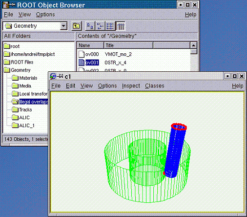
A volume containment region is in fact the result of the subtraction of all daughters. On the other hand, there are two other categories of overlaps that are considered illegal since they lead to unpredictable results during tracking.
If a positioned volume contains points that are not also contained by its mother, we will call the corresponding region as an extrusion. When navigating from outside to inside (trying to enter such a node) these regions are invisible since the current track has not yet reached its mother. This is not the case when going the other way since the track has first to exit the extruding node before checking the mother. In other words, an extrusion behavior is dependent on the track parameters, which is a highly undesirable effect.
We will call overlaps only the regions in space contained by more than one node inside the same container. The owner of such regions cannot be determined based on hierarchical considerations; therefore they will be considered as belonging to the node from which the current track is coming from.
When coming from their container, the ownership is totally unpredictable. Again, the ownership of overlapping regions highly depends on the current track parameters.
We must say that even the overlaps of type A) and B) are allowed in case the corresponding nodes are created using TGeoVolume::AddNodeOverlap() method. Navigation is performed in such cases by giving priority to the non-overlapping nodes. The modeller has to perform an additional search through the overlapping candidates. These are detected automatically during the geometry closing procedure in order to optimize the algorithm, but we will stress that extensive usage of this feature leads to a drastic deterioration of performance. In the following we will focus on the non-declared overlaps of type A) and B) since this is the main source of errors during tracking. These are generally non-intended overlaps due to coding mistakes or bad geometry design. The checking package is loaded together with the painter classes and contains an automated overlap checker.**
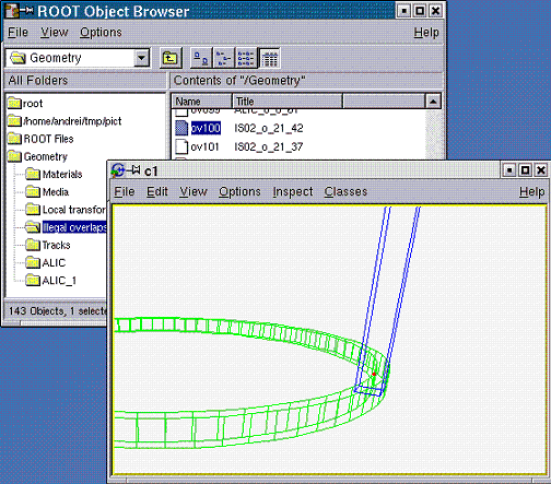
This can be activated both at volume level (checking for illegal overlaps only one level inside a given volume) and from the geometry manager level (checking full geometry):
myVolume->CheckOverlaps(precision, option);
gGeoManager->CheckOverlaps(precision);
myNode->CheckOverlaps(precision);
Here precision represents the desired maximum accepted overlap value in centimeters (default value is 0.1). This tool checks all possible significant pairs of candidates inside a given volume (not declared as overlapping or division volumes). The check is performed by verifying the mesh representation of one candidate against the shape of the other. This sort of check cannot identify all possible overlapping topologies, but it works for more than 95% and is much faster than the usual shape-to-shape comparison. For a 100% reliability, one can perform the check at the level of a single volume by using option=“d” or option=“d<number>” to perform overlap checking by sampling the volume with <number> random points (default 1 million). This produces also a picture showing in red the overlapping region and estimates the volume of the overlaps.
An extrusion A) is declared in any of the following cases:
An overlap B) is declared if:
The code is highly optimized to avoid checking candidates that are far away in space by performing a fast check on their bounding boxes. Once the checking tool is fired-up inside a volume or at top level, the list of overlaps (visible as Illegal overlaps inside a TBrowser) held by the manager class will be filled with TGeoOverlap objects containing a full description of the detected overlaps. The list is sorted in the decreasing order of the overlapping distance, extrusions coming first. An overlap object name represents the full description of the overlap, containing both candidate node names and a letter (x-extrusion, o-overlap) representing the type. Double-clicking an overlap item in a TBrowser produces a picture of the overlap containing only the two overlapping nodes (one in blue and one in green) and having the critical vertices represented by red points. The picture can be rotated/zoomed or drawn in X3d as any other view. Calling gGeoManager->PrintOverlaps() prints the list of overlaps.

In order to check a given point, CheckPoint(x,y,z) method of TGeoManager draws the daughters of the volume containing the point one level down, printing the path to the deepest physical node holding this point. It also computes the closest distance to any boundary.
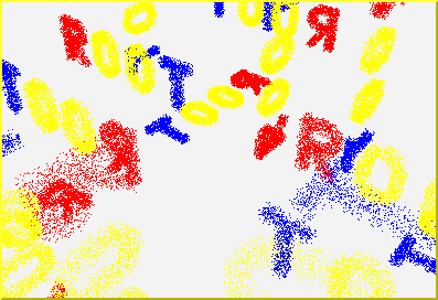
A method to check the validity of a given geometry is shooting random points. This can be called with the method TGeoVolume::RandomPoints() and it draws a volume with the current visualization settings. Random points are generated in the bounding box of the drawn volume. The points are drawn with the color of their deepest container. Only points inside visible nodes are drawn.
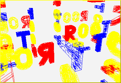
A ray tracing method can be called TGeoVolume::RandomRays(). This shoots rays from a given point in the local reference frame with random directions. The intersections with displayed nodes appear as segments having the color of the touched node.
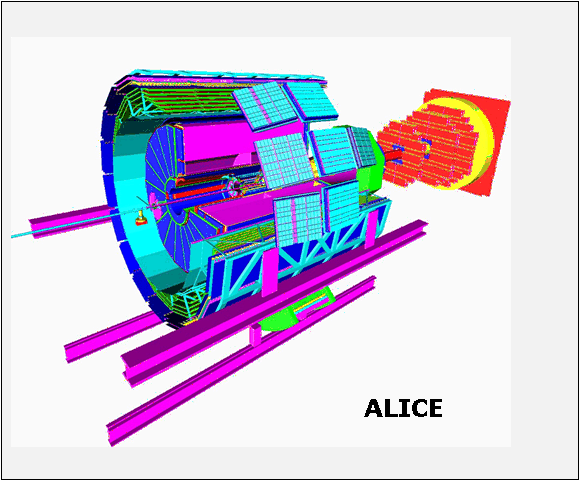 The modeller provides a powerful drawing package, supporting several different options of visualization. A library separated from the main one provides all functionality being linked with the underlying ROOT visualization system. This library is dynamically loaded by the plug-in manager only when drawing features are requested. The geometrical structures that can be visualized are volumes and volume hierarchies.
The main component of the visualization system is volume primitive painting in a ROOT pad. Starting from this one, several specific options or subsystems are available, like: X3D viewing using hidden line and surface removal algorithms, OpenGL viewing* or ray tracing.
The method TGeoManager::GetGeomPainter()loads the painting library in memory.
This is generally not needed since it is called automatically by TGeoVolume::Draw() as well as by few other methods setting visualization attributes.
The first thing one would like to do after building some geometry is to visualize the volume tree. This provides the fastest validation check for most common coding or design mistakes. As soon as the geometry is successfully closed, one should draw it starting from the top-level volume:
//... code for geometry building
root[] gGeoManager->CloseGeometry();
root[] gGeoManager->GetMasterVolume()->Draw();
Doing this ensures that the original top-level volume of the geometry is drawn, even if another volume is currently the geometry root. OK, I suppose you already did that with your simple geometry and immediately noticed a new ROOT canvas popping-up and having some more or less strange picture inside. Here are few questions that might come:
Q: “The picture is strangely rotated; where are the coordinate axes?”
A: If drawn in a new canvas, any view has some default viewpoint, center of view and size. One can then perform mouse/keyboard actions to change them:
Mouse left-click and drag will rotate the view;
Some keys can be pressed when the view canvas is selected: J/K zoom/un-zoom, U/I move up/down, L/H move left/right. The coordinate axes display as well as changing top or side viewpoints can be activated from the TView context menu: right-click on the picture when no object is selected;
Q: “Every line is black! I cannot figure out what is what…”
A: Volumes can have different colors (those known by ROOT of course). Think at using them after each volume creation: myvolume->SetLineColor(Int_t color); otherwise everything is by default black.
Q: “The top volume of my geometry is a box but I see only its content.”
A: By default the drawn volume is not displayed just because we do not want to hide its content when changing the view to HLR or solid mode. In order to see it in the default wire frame picture one has to call TGeoManager::SetTopVisible().
Q: “I do not see all volumes in my tree but just something inside.”
A: By default, TGeoVolume::Draw() paints the content of a given volume three levels down. You can change this by using: gGeoManager::SetVisLevel(n);
Not only that, but none of the volumes at intermediate levels (0-2) are visible on the drawing unless they are final ‘leaves’ on their branch (e.g. have no other volumes positioned inside). This behavior is the default one and corresponds to ‘leaves’ global visualization mode (TGeoManager::fVisOption = 1). In order to see on the screen the intermediate containers, one can change this mode: gGeoManager->SetVisOption(0).
Q: “Volumes are highlighted when moving the mouse over their vertices. What does it mean?”
A: Indeed, moving the mouse close to some volume vertices selects it. By checking the Event Status entry in the root canvas Options menu, you will see exactly which is the selected node in the bottom right. Right-clicking when a volume is selected will open its context menu where several actions can be performed (e.g. drawing it).
Q: “OK, but now I do not want to see all the geometry, but just a particular volume and its content. How can I do this?”
A: Once you have set a convenient global visualization option and level, what you need is just call the Draw() method of your interesting volume. You can do this either by interacting with the expanded tree of volumes in a ROOT browser (where the context menu of any volume is available), either by getting a pointer to it (e.g. by name): gGeoManager->GetVolume("vol_name")->Draw();
Supposing you now understand the basic things to do for drawing the geometry or parts of it, you still might be not happy and wishing to have more control on it. We will describe below how you can fine-tune some settings. Since the corresponding attributes are flags belonging to volume and node objects, you can change them at any time (even when the picture is already drawn) and see immediately the result.
We have already described how to change the line colors for volumes. In fact, volume objects inherit from TAttLine class so the line style or width can also be changed:
When drawing in solid mode, the color of the drawn volume corresponds to the line color.
The way geometry is build forces the definition of several volumes that does not represent real objects, but just virtual containers used for grouping and positioning volumes together. One would not want to see them in the picture. Since every volume is by default visible, one has to do this sort of tuning by its own:
As described before, the drawing package supports two main global options: 1 (default) - only final volume leaves; 0 - all volumes down the drawn one appear on the screen. The global visible level put a limitation on the maximum applied depth. Combined with visibility settings per volume, these can tune quite well what should appear on the screen. However, there are situations when users want to see a volume branch displayed down to the maximum depth, keeping at the same time a limitation or even suppressing others. In order to accomplish that, one should use the volume attribute: Visible daughters. By default, all daughters of all volumes are displayed if there is no limitation related with their level depth with respect to the top drawn volume.
Ray tracing is a quite known drawing technique based on tracking rays from the eye position through all pixels of a view port device. The pixel color is derived from the properties of the first crossed surface, according some illumination model and material optical properties. While there are currently existing quite sophisticated ray tracing models, TGeo is currently using a very simple approach where the light source is matching the eye position (no shadows or back-tracing of the reflected ray). In future we are considering providing a base class in order to be able to derive more complex models.
Due to the fact that the number of rays that have to be tracked matches the size in pixels of the pad, the time required by this algorithm is proportional to the pad size. On the other hand, the speed is quite acceptable for the default ROOT pad size and the images produced by using this technique have high quality. Since the algorithm is practically using all navigation features, producing ray-traced pictures is also a geometry validation check. Ray tracing can be activated at volume level as the normal Draw().
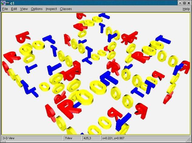
Once ray-tracing a view, this can be zoomed or rotated as a usual one. Objects on the screen are no longer highlighted when picking the vertices but the corresponding volumes is still accessible.
A ray-traced view can be clipped with any shape known by the modeller. This means that the region inside the clipping shape is subtracted from the current drawn geometry (become invisible). In order to activate clipping, one has to first define the clipping shape(s):
1. TGeoShape *clip1, *clip2, ...
One might switch between several clipping shapes. Note that these shapes are considered defined in the current MARS. Composite shapes may be used.
2. gGeoManager->SetClippingShape(clip1);
One can activate or deactivate clipping at any time: gGeoManager->SetClipping(flag);
gGeoManager->GetTopVolume()->Raytrace();One can redo the steps 2-3 as many times as needed. Let us look how the rootgeom example looks clipped with a tube.
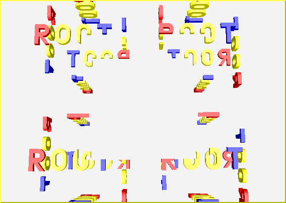
The ideal positioning of a detector does not match its position in the experimental hall. This generally happens not only for the detector modules, but also for their components. The accurate knowledge of the detector real misalignments can be extremely important for getting close to its designed resolution and the expected tracking efficiency. TGeo offers tools for representing positioning misalignments, applying them to the ideal geometry and performing navigation under these conditions. Detector tracking algorithms can then directly query the geometry for navigation purposes or for retrieving actual misalignment information.
Physical nodes are the actual “touchable” objects in the geometry, representing actually a path of positioned volumes starting with the top node: path=/TOP/A_1/B_4/C_3 , where A, B, C represent names of volumes. The number of physical nodes is given by the total number of possible of branches in the geometry hierarchy. In case of detector geometries and specially for calorimeters this number can be of the order 106-109, therefore it is impossible to create all physical nodes as objects in memory. In TGeo, physical nodes are represented by the class TGeoPhysicalNode and can be created on demand for alignment purposes:
The knowledge of the path to the objects that need to be misaligned is essential since there is no other way of identifying them. One can however create “symbolic links” to any complex path to make it more representable for the object it designates:
TGeoPNEntry(const char* unique_name, const char* path)
void TGeoPNEntry::SetPhysicalNode(TGeoPhysicalNode *node)
Such a symbolic link hides the complexity of the path to the align object and replaces it with a more meaningful name. In addition, TGeoPNEntry objects are faster to search by name and they may optionally store an additional user matrix.
// Creating a symlink object.
TGeoPNEntry *TGeoManager::SetAlignableEntry(const char *unique_n,
const char*path)
// Retrieving an existing alignable object.
TGeoPNEntry *TGeoManager::GetAlignableEntry(const char *name)
// Retrieving an existing alignable object at a given index.
TGeoPNEntry *GetAlignableEntry(Int_t index)
Physical nodes store internally the full list of logical nodes corresponding to the elements from the string path, as well as the global transformation matrix for each of them. The top node corresponds to the level 0 in the stored array, while the last node will correspond to level n. For each level, the node, volume and global matrix can be retrieved using corresponding getters:
TGeoHMatrix *GetMatrix(Int_t level=-1) const
TGeoNode    *GetNode(Int_t level=-1) const
TGeoShape   *GetShape(Int_t level=-1) const
TGeoVolume  *GetVolume(Int_t level=-1) const
By default the object at level n is retrieved (the align-able object).
Once created, a physical node can be misaligned, meaning that its positioning matrix or even the shape.:
The convention used is that newmat represents the new local matrix of the last node in the branch with respect to its mother volume. The Align() method will actually duplicate the corresponding branch within the logical hierarchy, creating new volumes and nodes. This is mandatory in order to avoid problems due to replicated volumes and can create exhaustive memory consumption if used abusively.
Once aligned, a physical node is ready to be tracked. The operation can be done only after the geometry was closed.
Important NOTE: Calling the Align() method for a physical node changes the node pointers for the stored node branch in the active geometry, Due to this the other defined physical nodes containing elements of this path will be invalid. Example:
TGeoPhysicalNode *pn1 =
gGeoManager->MakePhysicalNode("/A_1/B_1/C_2");
TGeoPhysicalNode *pn2 =
gGeoManager->MakePhysicalNode("/A_1/B_1/C_3");
...
pn1->Align(...);
The call to pn1->Align() will invalidate the pointer to the node B_1 in pn2 object.. The way out is to either call pn1->Align() before the creation of pn2, either to use a global method that will correct all existing physical nodes:
The method above will optionally lock the possibility of doing any further misalignment.
Once geometry is successfully built, it can be saved in a root file, as C++ macro or as GDML file by calling:
Filenameis the name of the file to be written (mandatory). Depending on the extension of the file, the geometry is exported either as ,root file or .C(.cxx) macro or GDML file in case extension is .gdml.keynameis the name of the key in the file (default "")opt = "v" is an export voxelization (default), otherwise voxelization is recomputed after loading the geometry, "g" this option (default) is taken into account only for exporting to gdml file and it ensures compatibility with Geant4 (e.g. it adds extra plane to incorrectly set polycone, it checks whether offset of Phi division is in (-360;0> range, …), for this gdml export there are two more option, that are not set by default: "f" and "n". If none of this two options are set, then names of solids and volumes in resulting gdml file will have incremental suffix (e.g. TGeoBBox_0x1, TGeoBBox_0x2, …). If "f" option is set then then suffix will contain pointer of object (e.g. TGeoBBox_0xAAAAA01, …). Finally if option "n" is set then no suffix will be added, though in this case uniqueness of the names is not ensured and it can cause that file will be invalid.Loading geometry from a root file can be done in the same way as for any other ROOT object, but a static method is also provided:
Example:
// Writing to a file geometry definition ending with:
root[] gGeoManager->CloseGeometry();
// geometry is ready
root[] gGeoManager->Export("MyGeom.root");
// file MyGeom.root produced
root[] gGeoManager->Export("MyGeom.C");
 // C++ macro MyGeom.C produced
root[] gGeoManager->Export("MyGeom.gdml");
 // GDML file MyGeom.gdml produced
root[] myVolume->SaveAs("MyVolume.C");
 // C++ macro for the branch starting
 // with MyVolume
// Reading from a file
root[] gSystem->Load("libGeom");
root[] TGeoManager::Import("MyGeom.root");  // geometry is ready
Note that not all-current information held by the modeller is written on the file. For instance, the painter and checker objects are not written, as well as the temporary current navigation properties: current node path, point or direction. On the other hand, all objects belonging to the geometrical hierarchy will always be written. The idea is to be able to retrieve the geometry in a ready state, ignoring what the state variables that can be always re-initialized. When the code is generated for a given TGeoVolume in the geometry, just the branch starting with that volume will be saved in the file. Executing the generated code will create a geometry that has MyVolume as top volume. In this case, only the materials/media/matrices used effectively in the MyVolume branch are exported to file.
Volumes can be made persistent in the same way the full geometry is. Exporting is straightforward (module1, 2 are pointers to TGeoVolume objects):
module1->Export("file.root");
// by default file is overwritten
module2->Export("file.root","","update");
// to the same file
Importing will append the volume to the current TGeoManager or will create one:
TGeoManager *geom = new TGeoManager("myGeom", "");
TGeoVolume *top = geom->MakeBox(...);
geom->SetTopVolume(top);
//name of volume or key (depending on export usage)
TGeoVolume *module1 = TGeoVolume::Import("file.root", "MOD1");
TGeoVolume *module2 = TGeoVolume::Import("file.root", "MOD2");
top->AddNode(module1, 1, new TGeoTranslation(0,0,100));
top->AddNode(module2, 1, new TGeoTranslation(0,0,-100));
// One should close oneself the geometry
geom->CloseGeometry();Few lines above word GDML was used. GDML stands for Geometry Description Markup Language. It is an application-independent geometry description format based on XML. It is mainly used for geometry interchange between ROOT and Geant4 framework. More details about this project can be found http://gdml.web.cern.ch. This feature (importing/exporting from/to gdml file format) is disabled by default in ROOT installation. To enable this feature add --enable-gdml option to ./configure script call.
This section will describe the main methods and algorithms used for implementing the navigation features within the geometrical modeller. This includes navigation queries at shape level, global geometrical queries and optimization mechanisms.
For reminder, a geometry state is a ‘touchable’ object in the geometry hierarchy. It is represented by a path like: /TOP_1/A_1/B_3/C_1, where B_3 for instance is a copy of volume B positioned inside volume A. A state is always associated to a transformation matrix M of the touchable with respect to the global reference frame (obtained by piling-up all local transformations of nodes in the branch with respect to their containers). The current state and the corresponding global matrix are updated whenever the geometry depth is modified. The global transformations corresponding to all nodes in the current branch are kept in an array: (MTOP_1, MA_1, MB_3, …).
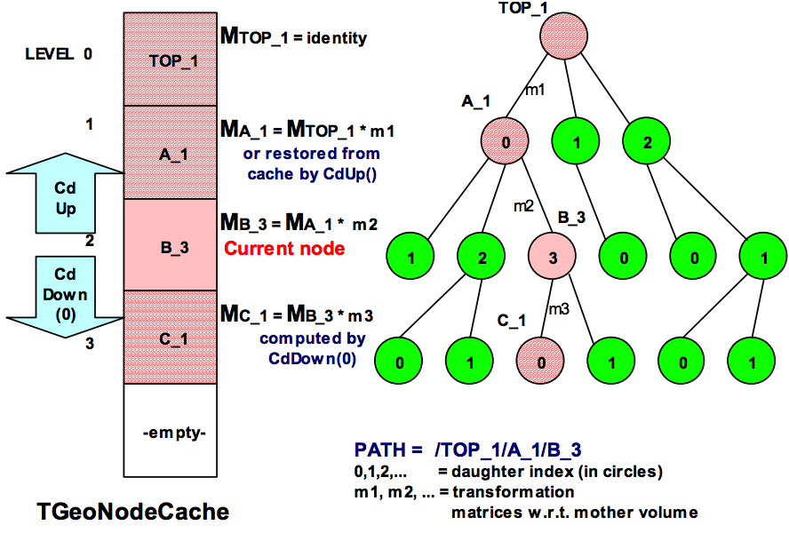
The elementary operations for changing the state are:
The current state accounting and global matrix handling after these operations are depicted in the figure below. Now let us suppose that we have a particle at position P(x,y,z). The first thing needed for transporting it is the current object our particle is into, so that we can retrieve its material properties. This task is done by:
Note that the current particle position can be set using SetCurrentPosition(x,y,z) method of the manager class, in which case FindNode() can be called without arguments. The method returns a pointer to the deepest node that geometrically contains P (in our case let us suppose it is B_3). Since a node is just a positioned volume, we can then get a pointer to the volume, medium or material objects related to it. Deepest means that B_3 still contains point P (as well as A_1 and TOP_1), but none of the daughters of volume B does. After finding out the node containing the particle, one can check if the geometry state is different compared to the last located point:
The algorithm for finding where a point is located in geometry is presented in the figure 17-36.
It always starts by checking if the last computed modeller state is the answer. This optimizes the search when continuously tracking a particle. The main actions performed are:
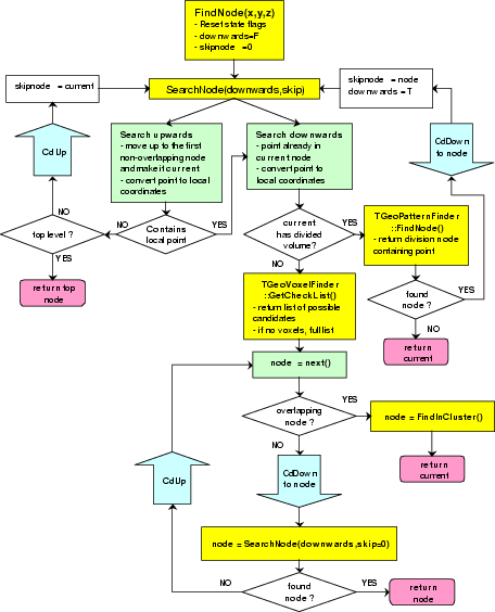
The most important feature provided by the modeller related to track propagation is the computation of the distance to the next boundary along a straight line.
The relevant state parameters used for this task are:
(x,y,z,nx,ny,nz), where ni is the direction cosine with axis (i).TGeoManager::FindNode(x,y,z)beforehand The method computing the distance to next boundary is:The output node returned by the method is the object which shape boundary will be crossed first. The distance to the next crossing can be retrieved after the call:
stepmax, which act as a trigger for different features. The absolute value of this parameter represents the step value proposed by the user. The algorithm will never try o search for boundaries further than this distance. In case no boundary is found the returned node will be the current one and the computed step to boundary will be equal to abs (stepmax) having the meaning “step approved”. The default value for stepmax is TGeoShape::Bigwith the meaning that boundaries are looked for without limitation.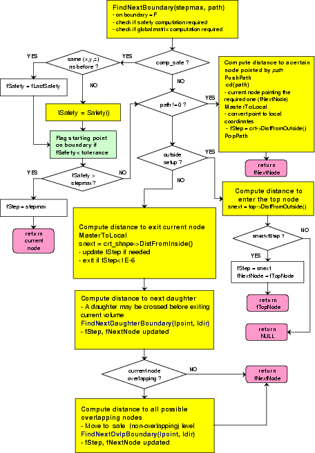
According the values of the input parameters the method will perform additional optional tasks:
|stepmax| < TGeoShape::Big()
The safe distance in the current volume is also computed. Moving the particle from its current location with this distance in any direction is safe in the sense that will never change the current state.
stepmax < 0
The global matrix for the object that will have the next crossed boundary is also computed. This can be retrieved for masterlocal point or vector conversions: TGeoManager::GetNextMatrix()
In case the computation of the normal vector to the next crossed surface is required, using a negative stepmax value is recommended. In this case one can subsequently call a method for fast normal computation:
path 0
In case a path to a given physical object is specified, the distance to its boundary is computed ignoring the rest of the geometry
TGeoManager::GetStep(): distance to next boundary.
TGeoManager::GetSafeDistance(): safe distance (in case it was computed).
TGeoManager::IsOnBoundary(): the initial point (x,y,z) was (or was not) on a boundary within TGeoShape::Tolerance().
The algorithm checks first if the computation of safety was required. If this is the case and the global point coordinates did not change from the last query, the last computed safety is taken. Otherwise, the method TGeoManager::Safety () is invoked. A safety value less than TGeoShape::Tolerance() will set the flag IsOnBoundary to true. On the other hand, a safety value bigger than the proposed step will stop the computation of the distance to next boundary, returning the current geometry location with the meaning that the proposed step is safe.
The next stage is to check if computation of the distance to a give physical object specified by a path was required. If this is the case, the modeller changes the state to point to the required object, converts the current point and direction coordinates to the local frame of this object and computes the distance to its shape. The node returned is the one pointed by the input path in case the shape is crossed; otherwise the returned value is NULL. In case the distance to next crossed boundary is required, the current point has to be physically INSIDE the shape pointed by the current volume. This is only insured in case a call to TGeoManager::FindNode() was performed for the current point. Therefore, the first step is to convert the global current point and direction in the local reference frame of the current volume and to compute the distance to exit its shape from inside. The returned value is again compared to the maximum allowed step (the proposed one) and in case the distance is safe no other action is performed and the proposed step is approved. In case the boundary is closer, the computed distance is taken as maximum allowed step. For optimization purposed, for particles starting very close to the current volume boundary (less than 0.01 microns) and exiting the algorithm stops here.
After computing the distance to exit the current node, the distance to the daughter of the current volume which is crossed next is computed by TGeoManager::FindNextDaughterBoundary(). This computes the distance to all daughter candidates that can be possibly crossed by using volume voxelization. The algorithm is efficient in average only in case the number of daughters is greater than 4. For fewer nodes, a simple loop is performed and the minimum distance (from a point outside each shape) is taken and compared to the maximum allowed step. The step value is again updated if step<stepmax .
A special case is when the current node is declared as possibly overlapping with something else. If this is the case, the distance is computed for all possibly overlapping candidates, taking into account the overlapping priorities (see also: " Overlapping volumes ").
The global matrix describing the next crossed physical node is systematically computed in case the value of the proposed step is negative. In this case, one can subsequently call TGeoManager::ComputeNormalFast() to get the normal vector to the crossed surface, after propagating the current point with the TGeoManager::GetStep() value. This propagation can be done like:
Double_t *current_point = gGeoManager->GetCurrentPoint();
Double_t *current_dir = gGeoManager->GetCurrentDirection();
for (Int_t i=0; i<3; i++)
    current_point[i] += step * current_dir[I];
Note: The method TGeoManager::FindNextBoundary() does not modify the current point/direction nor the current volume/state. The returned node is the next crossed one, but the physical path (state) AFTER crossing the boundary is not determined. In order to find out this new state, one has to propagate the point with a distance slightly bigger that the computed step value (which is accurate within numerical precision). A method that performs this task finding the next location is TGeoManager::Step(), described in " Making a Step ", but users may implement more precise methods to insure post-step boundary crossing.
The geombuilder package allows you to create and edit geometries. The package provides a library of all GUI classes related to geometry. Each editable geometry class TGeoXXX have a correspondent editor TGeoXXXEditor that provides a graphics user interface allowing to edit some (or all) parameters of a geometry object. The editable objects are geometry manager, volumes, nodes, shapes, media, materials and matrices. The interfaces provide also access to specific functionality of geometry objects. The editing mechanism is based on ROOT GED (Graphics Editors) functionality and the library is loaded using the plug-in mechanism.
There are two different use cases having different ways of invoking the geometry editors. The first one applies when starting with geometry from scratch and using the builder functionality to create new geometry objects. In this case, one should use the sequence:
root[] TGeoManager *geom = new TGeoManager("MyGeom",
"Test builder");
root[] geom->Edit(Option_t *option="");
The lines above will create a new TGeoManager class, create an empty canvas and start the editor in the left-sided editor frame attached to the canvas. To open the editor in a separate frame one should provide a non-empty string as option to the Edit() method.
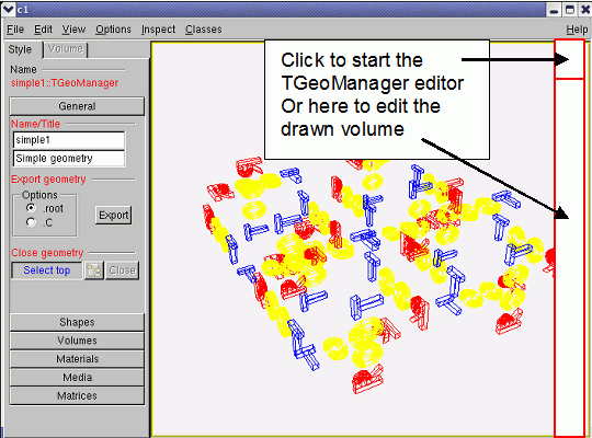
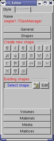
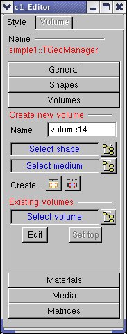
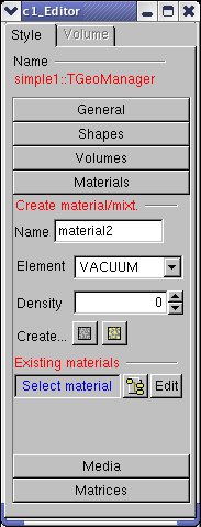
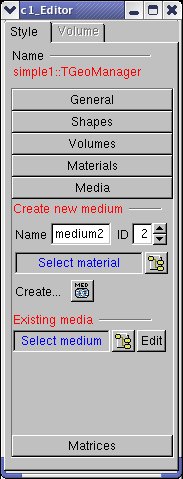
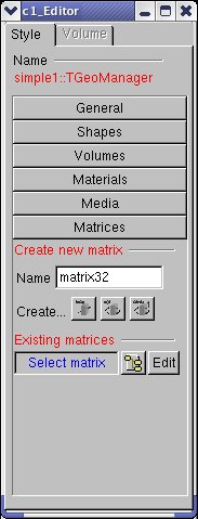
The second use case applies when starting to edit an existing geometry. Supposing the geometry was loaded into memory, besides the first method that still applies one can also edit drawn geometry objects. For this, the menu entry View/Editor of the canvas containing for instance a drawn volume must be activated. For starting the volume editor one can click on a volume. The GUI of the TGeoManager class can be started by clicking on the top-right 40x40 pixels corner of the pad with a drawn geometry.
This is the main entry point for editing the geometry or creating new objects. Once the interface is created (using one of the methods described above), several categories can be accessed via a shutter GUI widget:
geometry_name.C or .root depending if the geometry need to be saved as a C macro or a .root file.For editing an existing object from one of the categories described above, the interface imposes first a selection among all objects of the corresponding type stored in the geometry. This can be done by clicking the button next to the blue label Select <object>. The dialog interfaces are generally different for different types of objects. The volume selection dialog offers the possibility to select either a volume already connected to the geometry hierarchy or non-connected ones. Selection for shapes and matrices is split into categories represented by top-level list tree items for: boxes, tubes, translations, rotations, etc.
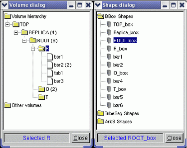
Once a selection is made and the dialog is closed, the selected item name will appear in the corresponding label and the button Edit will start the object editor in a transient frame. Closing these transient frames will not delete, but just hide existing opened editors for later reuse. Their lifetime is determined by the canvas to which the manager editor is attached to, since these will be destroyed together.
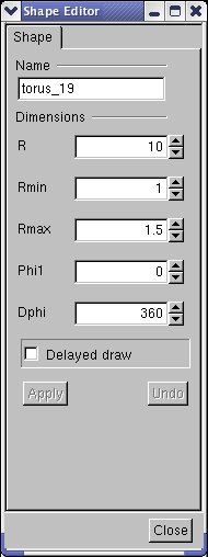
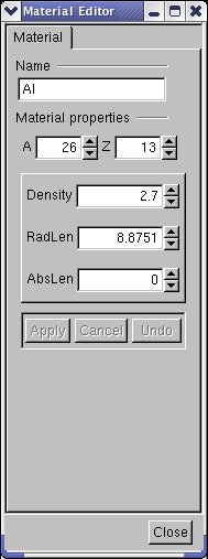
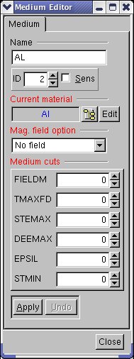
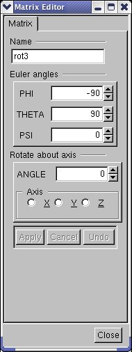
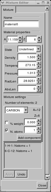
For most editors, the functionalities Apply and Undo are provided.
For shapes, changing any of the shape parameters will activate the “Apply” button only if the check button “Delayed draw” is checked, otherwise the changes are immediately applied. Once the apply button is pressed, the changes are applied to the edited shape and drawn. The “Undo” button becomes active after the first modification has been applied. It allows restoring the initial parameters of the shape.
NOTE: In this version the “Undo” does not allow restoring an intermediate state of the parameters that was applied - it will always restore the parameters at the moment the shape was edited.
All material properties changes are undoable. The mixture editor currently allows adding elements one by one in the mixture composition. This can be done either by element weight fraction or by number of atoms. Once an element was added using one method the other method is not selectable anymore. Summing component fractions up to 1 in the final mixture is the user responsibility. Adding materials as components of a mixture is not supported in this version.
The elements that were added to the mixture appear in the bottom of the mixture editor. The operations performed on mixture are not undoable.
As described above, all geometry object creators are accessible within the geometry manager editor frame. Generally, if the new object that needs to be created does not depend on other objects, it will be built with a set of default parameters. This is the case for all shapes (except composite shapes) and matrices. For all the other objects the interface forces the selection of components before creating the object.
Volumes are hierarchical components in the geometry, therefore their editor is more complex. It provides the following functionalities:
General. This category allows changing the name of the volume and selecting other shape or medium among existing ones.
Daughters. The category allows removing existing daughter nodes or adding new ones. The button “Position” allows editing the positioning matrix of a given node.

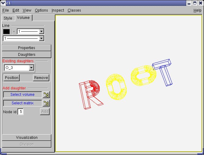
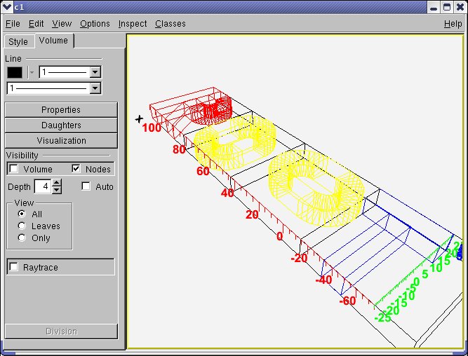
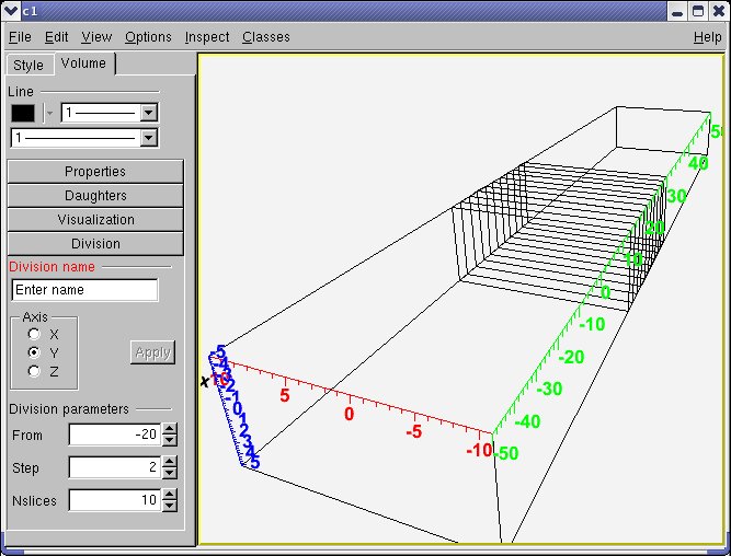
start and start+ndiv*step values and its validity is checked upon changing one of the values.NOTE: When changing a value in a number entry by typing a number, press ENTER at the end to validate. This applies for taking into account and validation of any number change in the geometry editors.
Create a new geometry manager and start the editor as described at the beginning.
Create at least one material from the “Materials” shutter item category. Generally, for creating objects, the interface is always in the TGeoManagerEditor in different categories - one should just provide a name and requested parameters.
Create a shape that will be used for the top volume within the “Shapes” category. For the moment, the shapes that have editors are Box, Para, Trd1, Trd2, Tube, Tube segment, Cone, Cone segment, Hype, Pcon, Torus and Sphere.
Create a medium from one of the existing materials from the “Medium” category. You will notice that some categories as “Volume” and “Medium” are inactive at the beginning because at that time there is no material yet (for making a medium) and no shape (for making a volume). These categories are dynamically activated once all the required components are defined.
Create a volume from the “Volumes” category. You will notice that contrary to the other editors, the volume editor is opened in a tab, not transient - this is because it is more complex.
Close the geometry from the “General” category.