WARNING: This documentation is not maintained anymore. Some part might be obsolete or wrong, some part might be missing but still some valuable information can be found there. Instead please refer to the ROOT Reference Guide and the ROOT Manual. If you think some information should be imported in the ROOT Reference Guide or in the ROOT Manual, please post your request to the ROOT Forum or via a Github Issue.
% Chapter: Graphs ________________________________________________________________________________________ WARNING: This documentation is not maintained anymore. Some part might be obsolete or wrong, some part might be missing but still some valuable information can be found there. Instead please refer to the ROOT Reference Guide and the ROOT Manual. If you think some information should be imported in the ROOT Reference Guide or in the ROOT Manual, please post your request to the ROOT Forum or via a Github Issue.
A graph is a graphics object made of two arrays X and Y, holding the x,y coordinates of n points. There are several graph classes; they are TGraph, TGraphErrors, TGraphAsymmErrors, and TMultiGraph.
The TGraph class supports the general case with non-equidistant points, and the special case with equidistant points. Graphs are created with the TGraph constructor. First, we define the arrays of coordinates and then create the graph. The coordinates can be arrays of doubles or floats.
   Int_t n = 20;
   Double_t x[n], y[n];
   for (Int_t i=0; i<n; i++) {
      x[i] = i*0.1;
      y[i] = 10*sin(x[i]+0.2);
   }
   TGraph *gr1 = new TGraph (n, x, y);
An alternative constructor takes only the number of points n. It is expected that the coordinates will be set later.
The default constructor can also be used. Further calls to SetPoint() will extend the internal vectors.
The various drawing options for a graph are explained in TGraph::PaintGraph. They are:
“L” A simple poly-line between every points is drawn
“F” A fill area is drawn
“F1” Idem as “F” but fill area is no more repartee around X=0 or Y=0
“F2” draw a fill area poly line connecting the center of bins
“A” Axis are drawn around the graph
“C” A smooth curve is drawn
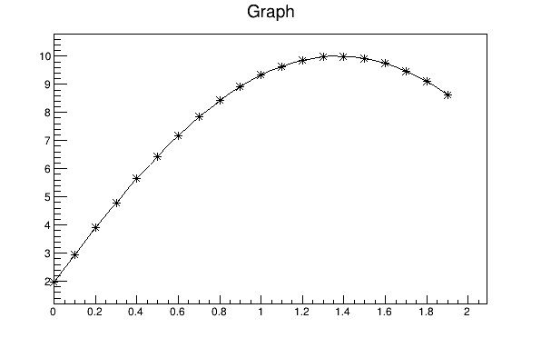
“*” A star is plotted at each point
“P” The current marker of the graph is plotted at each point
“B” A bar chart is drawn at each point
“[]” Only the end vertical/horizontal lines of the error bars are drawn. This option only applies to the TGraphAsymmErrors.
“1” ylow = rwymin
The options are not case sensitive and they can be concatenated in most cases. Let us look at some examples.
{
   Int_t n = 20;
   Double_t x[n], y[n];
   for (Int_t i=0;i<n;i++) {
      x[i] = i*0.1;
      y[i] = 10*sin(x[i]+0.2);
   }

   // create graph
   TGraph *gr  = new TGraph(n,x,y);
   TCanvas *c1 = new TCanvas("c1","Graph Draw Options",
                             200,10,600,400);

   // draw the graph with axis, continuous line, and put
   // a * at each point
   gr->Draw("AC*");
}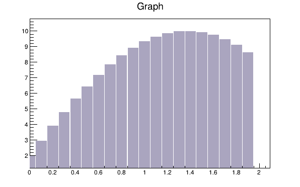
This code will only work if n, x, and y is defined. The previous example defines these. You need to set the fill color, because by default the fill color is white and will not be visible on a white canvas. You also need to give it an axis, or the bar chart will not be displayed properly.
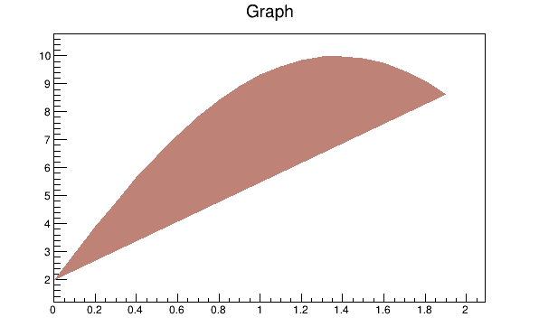
This code will only work if n, x, yare defined. The first example defines them. You need to set the fill color, because by default the fill color is white and will not be visible on a white canvas. You also need to give it an axis, or the filled polygon will not be displayed properly.
{
Int_t n = 20;
Double_t x[n], y[n];
// build the arrays with the coordinate of points
for (Int_t i=0; i<n; i++) {
x[i] = i*0.1;
y[i] = 10*sin(x[i]+0.2);
}
// create graphs
TGraph *gr3 = new TGraph(n,x,y);
TCanvas *c1 = new TCanvas ("c1","Graph Draw Options",
200,10,600,400);
// draw the graph with the axis,contineous line, and put
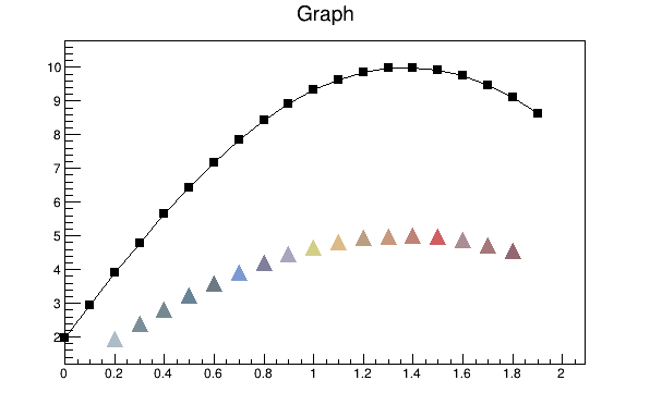
// a marker using the graph's marker style at each point
gr3->SetMarkerStyle(21);
c1->cd(4);
gr3->Draw("APL");
// get the points in the graph and put them into an array
Double_t *nx = gr3->GetX();
Double_t *ny = gr3->GetY();
// create markers of different colors
for (Int_t j=2; j<n-1; j++) {
TMarker *m = new TMarker(nx[j], 0.5*ny[j], 22);
m->SetMarkerSize(2);
m->SetMarkerColor(31+j);
m->Draw();
}
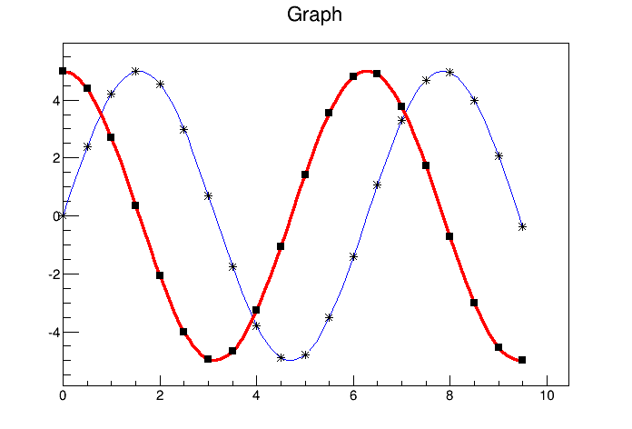
}To super impose two graphs you need to draw the axis only once, and leave out the “A” in the draw options for the second graph. Next is an example:
{
   Int_t n = 20;
   Double_t x[n], y[n], x1[n], y1[n];

   // create a blue graph with a cos function
   gr1->SetLineColor(4);
   gr1->Draw("AC*");

   // superimpose the second graph by leaving out the axis option "A"
   gr2->SetLineWidth(3);
   gr2->SetMarkerStyle(21);
   gr2->SetLineColor(2);
   gr2->Draw("CP");
}A TGraphErrors is a TGraph with error bars. The various draw format options of TGraphErrors::Paint() are derived from TGraph.
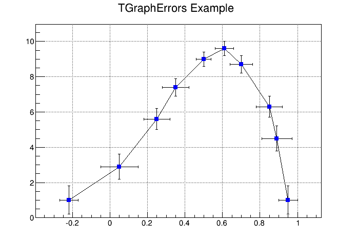
In addition, it can be drawn with the “Z” option to leave off the small lines at the end of the error bars. If option contains “>”, an arrow is drawn at the end of the error bars. If option contains “|>”, a full arrow is drawn at the end of the error bars. The size of the arrow is set to 2/3 of the marker size.
The option “[]” is interesting to superimpose systematic errors on top of the graph with the statistical errors. When it is specified, only the end vertical/horizontal lines of the error bars are drawn.
To control the size of the lines at the end of the error bars (when option 1 is chosen) use SetEndErrorSize(np). By default np=1; np represents the number of pixels.
The four parameters of TGraphErrors are: X, Y (as in TGraph), X-errors, and Y-errors - the size of the errors in the x and y direction. Next example is $ROOTSYS/tutorials/visualisation/graphs/gerrors.C.
{
   c1 = new TCanvas("c1","A Simple Graph with error bars",200,10,700,500);
   c1->SetGrid();

   // create the coordinate arrays
   Int_t n = 10;
   Float_t x[n]  = {-.22,.05,.25,.35,.5,.61,.7,.85,.89,.95};
   Float_t y[n]  = {1,2.9,5.6,7.4,9,9.6,8.7,6.3,4.5,1};

   // create the error arrays
   Float_t ex[n] = {.05,.1,.07,.07,.04,.05,.06,.07,.08,.05};
   Float_t ey[n] = {.8,.7,.6,.5,.4,.4,.5,.6,.7,.8};

   // create the TGraphErrors and draw it
   gr = new TGraphErrors(n,x,y,ex,ey);
   gr->SetTitle("TGraphErrors Example");
   gr->SetMarkerColor(4);
   gr->SetMarkerStyle(21);
   gr->Draw("ALP");
   c1->Update();
}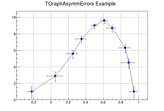
A TGraphAsymmErrors is a TGraph with asymmetric error bars. It inherits the various draw format options from TGraph. Its method Paint(Option_t *option) paints the TGraphAsymmErrors with the current attributes. You can set the following additional options for drawing:
“z” or “Z”the horizontal and vertical small lines are not drawn at the end of error bars
“>”an arrow is drawn at the end of the error bars
“|>”a full arrow is drawn at the end of the error bar; its size is \(\frac{2}{3}\) of the marker size
“[]”only the end vertical/horizontal lines of the error bars are drawn; this option is interesting to superimpose systematic errors on top of a graph with statistical errors.
The constructor has six arrays as parameters: X and Y as TGraph and low X-errors and high X-errors, low Y-errors and high Y-errors. The low value is the length of the error bar to the left and down, the high value is the length of the error bar to the right and up.
{
   c1 = new TCanvas("c1","A Simple Graph with error bars",
                    200,10,700,500);
   c1->SetGrid();

   // create the arrays for the points
   Int_t n = 10;
   Double_t x[n]  = {-.22,.05,.25,.35,.5, .61,.7,.85,.89,.95};
   Double_t y[n]  = {1,2.9,5.6,7.4,9,9.6,8.7,6.3,4.5,1};

   // create the arrays with high and low errors
   Double_t exl[n] = {.05,.1,.07,.07,.04,.05,.06,.07,.08,.05};
   Double_t eyl[n] = {.8,.7,.6,.5,.4,.4,.5,.6,.7,.8};
   Double_t exh[n] = {.02,.08,.05,.05,.03,.03,.04,.05,.06,.03};
   Double_t eyh[n] = {.6,.5,.4,.3,.2,.2,.3,.4,.5,.6};

   // create TGraphAsymmErrors with the arrays
   gr = new TGraphAsymmErrors(n,x,y,exl,exh,eyl,eyh);
   gr->SetTitle("TGraphAsymmErrors Example");
   gr->SetMarkerColor(4);
   gr->SetMarkerStyle(21);
   gr->Draw("ALP");
}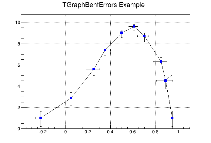
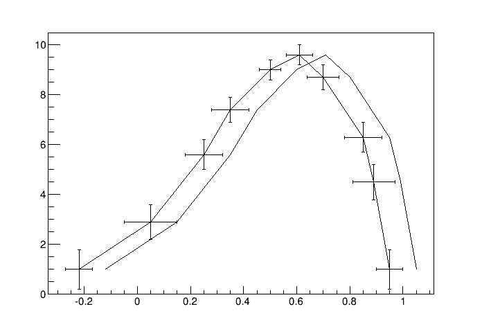
A TGraphBentErrors is a TGraph with bent, asymmetric error bars. The various format options to draw a TGraphBentErrors are explained in TGraphBentErrors::Paint method. The TGraphBentErrors is drawn by default with error bars and small horizontal and vertical lines at the end of the error bars. If option “z” or “Z” is specified, these small lines are not drawn. If the option “X” is specified, the errors are not drawn (the TGraph::Paint method equivalent).
if option contains “>”, an arrow is drawn at the end of the error bars
if option contains “|>”, a full arrow is drawn at the end of the error bars
the size of the arrow is set to 2/3 of the marker size
if option “[]” is specified, only the end vertical/horizontal lines of the error bars are drawn. This option is interesting to superimpose systematic errors on top of a graph with statistical errors.
This figure has been generated by the following macro:
{
   Int_t n = 10;
   Double_t x[n] = {-0.22,0.05,0.25,0.35,0.5,0.61,0.7,0.85,0.89,0.95};
   Double_t y[n] = {1,2.9,5.6,7.4,9,9.6,8.7,6.3,4.5,1};
   Double_t exl[n] = {.05,.1,.07,.07,.04,.05,.06,.07,.08,.05};
   Double_t eyl[n] = {.8,.7,.6,.5,.4,.4,.5,.6,.7,.8};
   Double_t exh[n] = {.02,.08,.05,.05,.03,.03,.04,.05,.06,.03};
   Double_t eyh[n] = {.6,.5,.4,.3,.2,.2,.3,.4,.5,.6};
   Double_t exld[n] = {.0,.0,.0,.0,.0,.0,.0,.0,.0,.0};
   Double_t eyld[n] = {.0,.0,.0,.0,.0,.0,.0,.0,.0,.0};
   Double_t exhd[n] = {.0,.0,.0,.0,.0,.0,.0,.0,.0,.0};
   Double_t eyhd[n] = {.0,.0,.0,.0,.0,.0,.0,.0,.05,.0};
   gr = new TGraphBentErrors(n,x,y,
                             exl,exh,eyl,eyh,exld,exhd,eyld,eyhd);
   gr->SetTitle("TGraphBentErrors Example");
   gr->SetMarkerColor(4);
   gr->SetMarkerStyle(21);
   gr->Draw("ALP");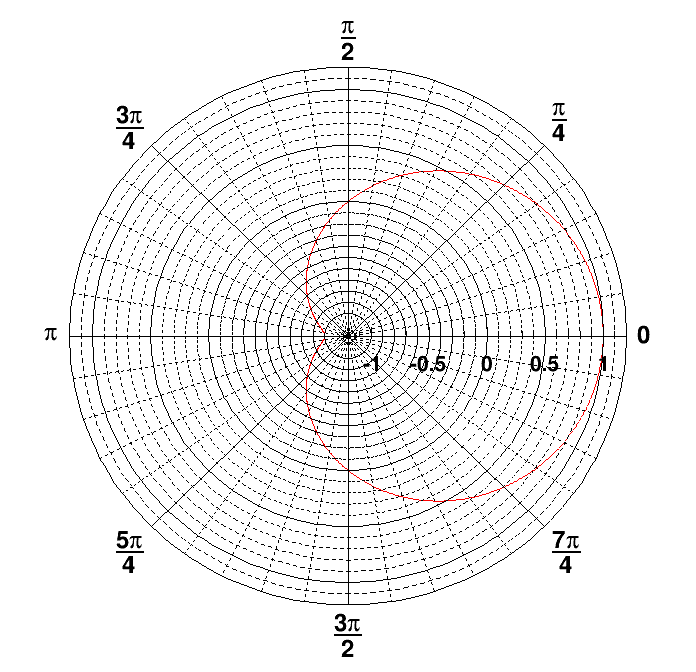
}The TGraphPolar class creates a polar graph (including error bars). A TGraphPolar is a TGraphErrors represented in polar coordinates. It uses the class TGraphPolargram to draw the polar axis.
{
   TCanvas *CPol = new TCanvas("CPol","TGraphPolar Examples",700,700);
   Double_t rmin=0;
   Double_t rmax=TMath::Pi()*2;
   Double_t r[1000];
   Double_t theta[1000];
   TF1 * fp1 = new TF1("fplot","cos(x)",rmin,rmax);
   for (Int_t ipt = 0; ipt < 1000; ipt++) {
      r[ipt] = ipt*(rmax-rmin)/1000+rmin;
      theta[ipt] = fp1->Eval(r[ipt]);
   }
   TGraphPolar * grP1 = new TGraphPolar(1000,r,theta);
   grP1->SetLineColor(2);
   grP1->Draw("AOL");
}
The TGraphPolar drawing options are:
“O” Polar labels are paint orthogonally to the polargram radius.
“P” Polymarker are paint at each point position.
“E” Paint error bars.
“F” Paint fill area (closed polygon).
“A”Force axis redrawing even if a polagram already exists.
When a graph is painted with the option “C” or “L”, it is possible to draw a filled area on one side of the line. This is useful to show exclusion zones. This drawing mode is activated when the absolute value of the graph line width (set thanks to SetLineWidth) is greater than 99. In that case the line width number is interpreted as 100*ff+ll = ffll. The two-digit numbers “ll” represent the normal line width whereas “ff” is the filled area width. The sign of “ffll” allows flipping the filled area from one side of the line to the other. The current fill area attributes are used to draw the hatched zone.
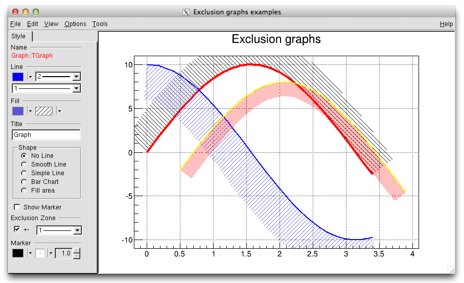
{
   c1 = new TCanvas("c1","Exclusion graphs examples",200,10,700,500);
   c1->SetGrid();

   // create the multigraph
   TMultiGraph *mg = new TMultiGraph();
   mg->SetTitle("Exclusion graphs");

   // create the graphs points
   const Int_t n = 35;
   Double_t x1[n], x2[n], x3[n], y1[n], y2[n], y3[n];
   for (Int_t i=0;i<n;i++) {
      x1[i] = i*0.1; y1[i] = 10*sin(x1[i]);
      x2[i] = x1[i]; y2[i] = 10*cos(x1[i]);
      x3[i] = x1[i]+.5; y3[i] = 10*sin(x1[i])-2;
   }

   // create the 1st TGraph
   gr1 = new TGraph(n,x1,y1);
   gr1->SetLineColor(2);
   gr1->SetLineWidth(1504);
   gr1->SetFillStyle(3005);

   // create the 2nd TGraph
   gr2 = new TGraph(n,x2,y2);
   gr2->SetLineColor(4);
   gr2->SetLineWidth(-2002);
   gr2->SetFillStyle(3004);
   gr2->SetFillColor(9);

   // create the 3rd TGraph
   gr3 = new TGraph(n,x3,y3);
   gr3->SetLineColor(5);
   gr3->SetLineWidth(-802);
   gr3->SetFillStyle(3002);
   gr3->SetFillColor(2);

   // put the graphs in the multigraph
   mg->Add(gr1);
   mg->Add(gr2);
   mg->Add(gr3);

   // draw the multigraph
   mg->Draw("AC");
}A TGraphQQ allows drawing quantile-quantile plots. Such plots can be drawn for two datasets, or for one dataset and a theoretical distribution function.
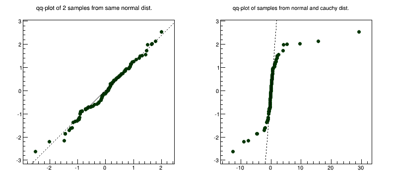
Quantile-quantile plots are used to determine whether two samples come from the same distribution. A qq-plot draws the quantiles of one dataset against the quantile of the other. The quantiles of the dataset with fewer entries are on Y-axis, with more entries - on X-axis. A straight line, going through 0.25 and 0.75 quantiles is also plotted for reference. It represents a robust linear fit, not sensitive to the extremes of the datasets. If the datasets come from the same distribution, points of the plot should fall approximately on the 45 degrees line. If they have the same distribution function, but different parameters of location or scale, they should still fall on the straight line, but not the 45 degrees one.
The greater their departure from the straight line, the more evidence there is that the datasets come from different distributions. The advantage of qq-plot is that it not only shows that the underlying distributions are different, but, unlike the analytical methods, it also gives information on the nature of this difference: heavier tails, different location/scale, different shape, etc.
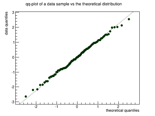
Quantile-quantile plots are used to determine if the dataset comes from the specified theoretical distribution, such as normal. A qq-plot draws quantiles of the dataset against quantiles of the specified theoretical distribution. Note, that density, not CDF should be specified a straight line, going through 0.25 and 0.75 quantiles could also be plotted for reference. It represents a robust linear fit, not sensitive to the extremes of the dataset. As in the two datasets case, departures from straight line indicate departures from the specified distribution. Next picture shows an example of a qq-plot of a dataset from N(3, 2) distribution and TMath::Gaus(0, 1) theoretical function. Fitting parameters are estimates of the distribution mean and sigma.
A TMultiGraph is a collection of TGraph (or derived) objects. Use TMultiGraph::Addto add a new graph to the list. The TMultiGraph owns the objects in the list. The drawing and fitting options are the same as for TGraph.
{
   // create the points
   Int_t n = 10;
   Double_t x[n]  = {-.22,.05,.25,.35,.5,.61,.7,.85,.89,.95};
   Double_t y[n]  = {1,2.9,5.6,7.4,9,9.6,8.7,6.3,4.5,1};
   Double_t x2[n]  = {-.12,.15,.35,.45,.6,.71,.8,.95,.99,1.05};
   Double_t y2[n]  = {1,2.9,5.6,7.4,9,9.6,8.7,6.3,4.5,1};

   // create the width of errors in x and y direction
   Double_t ex[n] = {.05,.1,.07,.07,.04,.05,.06,.07,.08,.05};
   Double_t ey[n] = {.8,.7,.6,.5,.4,.4,.5,.6,.7,.8};

   // create two graphs
   TGraph *gr1 = new TGraph(n,x2,y2);
   TGraphErrors *gr2 = new TGraphErrors(n,x,y,ex,ey);

   // create a multigraph and draw it
   TMultiGraph  *mg  = new TMultiGraph();
   mg->Add(gr1);
   mg->Add(gr2);
   mg->Draw("ALP");
}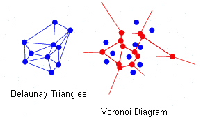
This class is a set of N points x[i], y[i], z[i] in a non-uniform grid. Several visualization techniques are implemented, including Delaunay triangulation. Delaunay triangulation is defined as follow: ‘for a set S of points in the Euclidean plane, the unique triangulation DT(S) of S such that no point in S is inside the circum-circle of any triangle in DT(S). DT(S) is the dual of the Voronoï diagram of S. If n is the number of points in S, the Voronoï diagram of S is the partitioning of the plane containing S points into n convex polygons such that each polygon contains exactly one point and every point in a given polygon is closer to its central point than to any other. A Voronoï diagram is sometimes also known as a Dirichlet tessellation.
The TGraph2D class has the following constructors:
n and three arrays x, y, and z (can be arrays of doubles, floats, or integers):SetPoint at the position “i” with the values x, y, z:SetPoint must be used to fill the internal arrays.The arrays are read from the ASCII file “graph.dat” according to a specified format. The format’s default value is “%lg %lg %lg”. Note that in any of last three cases, the SetPoint method can be used to change a data point or to add a new one. If the data point index (i) is greater than the size of the internal arrays, they are automatically extended.
Specific drawing options can be used to paint a TGraph2D:
“TRI” the Delaunay triangles are drawn using filled area. A hidden surface drawing technique is used. The surface is painted with the current fill area color. The edges of the triangles are painted with the current line color;
“TRIW”the Delaunay triangles are drawn as wire frame;
“TRI1” the Delaunay triangles are painted with color levels. The edges of the triangles are painted with the current line color;
“TRI2” the Delaunay triangles are painted with color levels;
“P”draws a marker at each vertex;
“P0” draws a circle at each vertex. Each circle background is white.
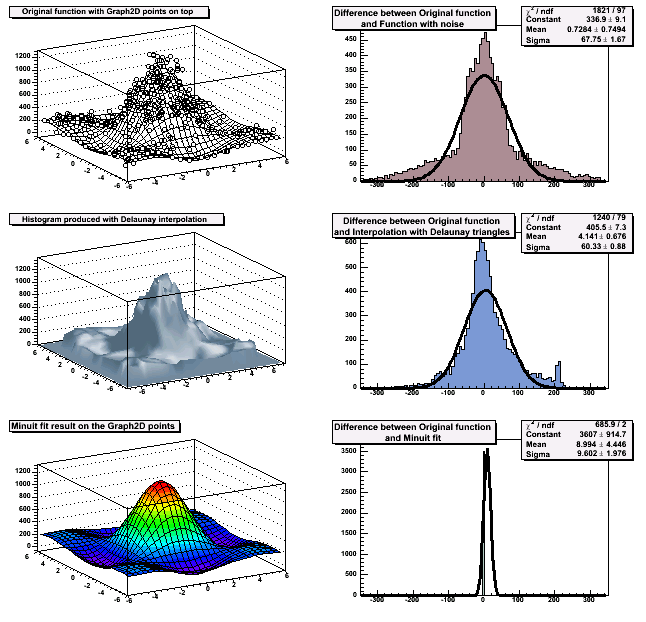
A TGraph2D can be also drawn with ANY options valid for 2D histogram drawing. In this case, an intermediate 2D histogram is filled using the Delaunay triangles technique to interpolate the data set. TGraph2D linearly interpolate a Z value for any (X,Y) point given some existing (X,Y,Z) points. The existing (X,Y,Z) points can be randomly scattered. The algorithm works by joining the existing points to make Delaunay triangles in (X,Y). These are then used to define flat planes in (X,Y,Z) over which to interpolate. The interpolated surface thus takes the form of tessellating triangles at various angles. Output can take the form of a 2D histogram or a vector. The triangles found can be drawn in 3D. This software cannot be guaranteed to work under all circumstances. It was originally written to work with a few hundred points in anXY space with similar X and Y ranges.

{
   TCanvas *c = new TCanvas("c","Graph2D example",0,0,700,600);
   Double_t x, y, z, P = 6.;
   Int_t np = 200;
   TGraph2D *dt = new TGraph2D();
   TRandom *r = new TRandom();

   for (Int_t N=0; N<np; N++) {
      x = 2*P*(r->Rndm(N))-P;
      y = 2*P*(r->Rndm(N))-P;
      z = (sin(x)/x)*(sin(y)/y)+0.2;
      dt->SetPoint(N,x,y,z);
   }
   gStyle->SetPalette(55);
   dt->Draw("surf1");       // use "surf1" to generate the left picture
}                           // use "tri1 p0" to generate the right one
A more complete example is $ROOTSYS/tutorials/fit/graph2dfit.C that produces the next figure.
A TGraph2DErrors is a TGraph2D with errors. It is useful to perform fits with errors on a 2D graph. An example is the macro $ROOTSYS/tutorials/visualisation/graphs/graph2derrorsfit.C.
The graph Fit method in general works the same way as the TH1::Fit. See “Fitting Histograms”.
To give the axis of a graph a title you need to draw the graph first, only then does it actually have an axis object. Once drawn, you set the title by getting the axis and calling the TAxis::SetTitle method, and if you want to center it, you can call the TAxis::CenterTitle method.
Assuming that n, x, and y are defined. Next code sets the titles of the x and y axes.
root[] gr5 = new TGraph(n,x,y)
root[] gr5->Draw()
<TCanvas::MakeDefCanvas>: created default TCanvas with name c1
root[] gr5->Draw("ALP")
root[] gr5->GetXaxis()->SetTitle("X-Axis")
root[] gr5->GetYaxis()->SetTitle("Y-Axis")
root[] gr5->GetXaxis()->CenterTitle()
root[] gr5->GetYaxis()->CenterTitle()
root[] gr5->Draw("ALP")
For more graph examples see the scripts: $ROOTSYS/tutorials directory graph.C, gerrors.C, zdemo.C, and gerrors2.C.

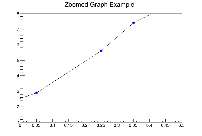
To zoom a graph you can create a histogram with the desired axis range first. Draw the empty histogram and then draw the graph using the existing axis from the histogram.
{
   c1 = new TCanvas("c1","A Zoomed Graph",200,10,700,500);
   hpx = new TH2F("hpx","Zoomed Graph Example",10,0,0.5,10,1.0,8.0);
   hpx->SetStats(kFALSE);   // no statistics
   hpx->Draw();
   Int_t n = 10;
   Double_t x[n] = {-.22,.05,.25,.35,.5,.61,.7,.85,.89,.95};
   Double_t y[n] = {1,2.9,5.6,7.4,9,9.6,8.7,6.3,4.5,1};
   gr = new TGraph(n,x,y);
   gr->SetMarkerColor(4);
   gr->SetMarkerStyle(20);
   gr->Draw("LP");// and draw it without an axis
}
The next example is the same graph as above with a zoom in the x and y directions.
The class TGraphEditor provides the user interface for setting the following graph attributes interactively:
Title text entry field … sets the title of the graph.
Shape radio button group - sets the graph shapes:
Show Marker - sets markers as visible or invisible.
Exclusion Zone - specifies the exclusion zone parameters :
