WARNING: This documentation is not maintained anymore. Some part might be obsolete or wrong, some part might be missing but still some valuable information can be found there. Instead please refer to the ROOT Reference Guide and the ROOT Manual. If you think some information should be imported in the ROOT Reference Guide or in the ROOT Manual, please post your request to the ROOT Forum or via a Github Issue.
The linear algebra package is supposed to give a complete environment in ROOT to perform calculations like equation solving and eigenvalue decompositions. Most calculations are performed in double precision. For backward compatibility, some classes are also provided in single precision like TMatrixF, TMatrixFSym and TVectorF. Copy constructors exist to transform these into their double precision equivalent, thereby allowing easy access to decomposition and eigenvalue classes, only available in double precision.
The choice was made not to provide the less frequently used complex matrix classes. If necessary, users can always reformulate the calculation in 2 parts, a real one and an imaginary part. Although, a linear equation involving complex numbers will take about a factor of 8 more computations, the alternative of introducing a set of complex classes in this non-template library would create a major maintenance challenge.
Another choice was to fill in both the upper-right corner and the bottom-left corner of a symmetric matrix. Although most algorithms use only the upper-right corner, implementation of the different matrix views was more straightforward this way. When stored only the upper-right part is written to file.
For a detailed description of the interface, the user should look at the root reference guide at: http://root.cern.ch/root/Reference.html
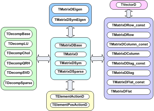
The figure below shows an overview of the classes available in the linear algebra library,libMatrix.so. At the center is the base class TMatrixDBase from which three different matrix classes, TMatrixD, TMatrixDSym and TMatrixDFSparse derive. The user can define customized matrix operations through the classes TElementActionD and TElementsPosActionD.
Reference to different views of the matrix can be created through the classes on the right-hand side, see “Matrix Views”. These references provide a natural connection to vectors.
Matrix decompositions (used in equation solving and matrix inversion) are available through the classes on the left-hand side (see “Matrix Decompositions”). They inherit from the TDecompBase class. The Eigen Analysis is performed through the classes at the top, see “Matrix Eigen Analysis”. In both cases, only some matrix types can be analyzed. For instance, TDecompChol will only accept symmetric matrices as defined TMatrixDSym. The assignment operator behaves somewhat different than of most other classes. The following lines will result in an error:
It required to first resize matrix b to the shape of a.
A matrix has five properties, which are all set in the constructor:
precision - float or double. In the first case you will use the TMatrixF class family, in the latter case the TMatrixD one;
type - general (TMatrixD), symmetric (TMatrixDSym) or sparse (TMatrixDSparse);
size - number of rows and columns;
index - range start of row and column index. By default these start at zero;
sparse map - this property is only relevant for a sparse matrix. It indicates where elements are unequal zero.
The following table shows the methods to access the information about the relevant matrix property:
| Method | Descriptions |
Int_t GetRowLwb () |
row lower-bound index |
Int_t GetRowUpb () |
row upper-bound index |
Int_t GetNrows () |
number of rows |
Int_t GetColLwb () |
column lower-bound index |
Int_t GetColUpb () |
column upper-bound index |
Int_t GetNcols () |
number of columns |
Int_t GetNoElements () |
number of elements, for a dense matrix this equals: fNrows x fNcols |
Double_t GetTol () |
tolerance number which is used in decomposition operations |
Int_t *GetRowIndexArray () |
for sparse matrices, access to the row index of fNrows+1 entries |
Int_t *GetColIndexArray () |
for sparse matrices, access to the column index of fNelems entries |
The last two methods in this table are specific to the sparse matrix, which is implemented according to the Harwell-Boeing format. Here, besides the usual shape/size descriptors of the matrix like fNrows, fRowLwb, fNcols and fColLwb, we also store a row index, fRowIndex and column index, fColIndex for the elements unequal zero:
fRowIndex[0,..,fNrows]: |
Stores for each row the index range of the elements in the data and column array |
fColIndex[0,..,fNelems-1]: |
Stores the column number for each data element != 0. |
The code to print all matrix elements unequal zero would look like:
   TMatrixDSparse a;
   const Int_t *rIndex = a.GetRowIndexArray();
   const Int_t *cIndex = a.GetColIndexArray();
   const Double_t *pData = a.GetMatrixArray();
   for (Int_t irow = 0; irow < a.getNrows(); irow++) {
      const Int_t sIndex = rIndex[irow];
      const Int_t eIndex = rIndex[irow+1];
      for (Int_t index = sIndex; index < eIndex; index++) {
         const Int_t icol = cIndex[index];
         const Double_t data = pData[index];
         printf("data(%d,%d) = %.4en",irow+a.GetfRowLwb(),
         icol+a.GetColLwb(),data);
      }
}The following table shows the methods to set some of the matrix properties. The resizing procedures will maintain the matrix elements that overlap with the old shape. The optional last argument nr_zeros is only relevant for sparse matrices. If supplied, it sets the number of non-zero elements. If it is smaller than the number overlapping with the old matrix, only the first (row-wise)nr_zeros are copied to the new matrix.
| Method | Descriptions |
|---|---|
SetTol (Double_t tol) |
set the tolerance number |
|
change matrix shape to nrows x ncols. Index will start at zero |
|
change matrix shape to
|
SetRowIndexArray (Int_t *data) |
for sparse matrices, set the row index. The array data should contains at leastfNrows+1 entries column lower-bound index |
SetColIndexArray (Int_t *data) |
for sparse matrices, set the column index. The array data should contains at least fNelems entries |
SetSparseIndex (Int_t nelems new) |
allocate memory for a sparse map of nelems_new elements and copy (if exists) at most nelems_new matrix elements over to the new structure |
SetSparseIndex (const TMatrixDBase &a) |
copy the sparse map from matrix a Note that this can be a dense matrix! |
SetSparseIndexAB (const TMatrixDSparse &a, const TMatrixDSparse &b) |
set the sparse map to the same of the map of matrix a and b |
The second half of the table is only relevant for sparse matrices. These methods define the sparse structure. It should be clear that a call to any of these methods has to be followed by a SetMatrixArray (…) which will supply the matrix data, see the next chapter “Creating and Filling a Matrix”.
The matrix constructors are listed in the next table. In the simplest ones, only the number of rows and columns is given. In a slightly more elaborate version, one can define the row and column index range. Finally, one can also define the matrix data in the constructor. In Matrix Operators and Methods we will encounter more fancy constructors that will allow arithmetic operations.
|
|
|
If only the matrix shape is defined in the constructor, matrix data has to be supplied and possibly the sparse structure. In “Setting Properties” was discussed how to set the sparse structure.
Several methods exist to fill a matrix with data:
SetMatrixArray(const Double_t*data,Option_t*option=""), copies the array data. If option="F", the array fills the matrix column-wise else row-wise. This option is only implemented for TMatrixD and TMatrixDSym. It is expected that the array data contains at least fNelems entries.
SetMatrixArray(Int_t nr,Int_t *irow,Int_t *icol,Double_t *data), is only available for sparse matrices. The three arrays should each contain nr entries with row index, column index and data entry. Only the entries with non-zero data value are inserted!
operator()or operator[], these operators provide the easiest way to fill a matrix but are in particular for a sparse matrix expensive. If no entry for slot (i,j) is found in the sparse index table it will be entered, which involves some memory management! Therefore, before invoking this method in a loop it is wise to set the index table first through a call to the SetSparseIndex method.
SetSub(Int_t row_lwb,Int_t col_lwb,const TMatrixDBase &source), the matrix to be inserted at position (row_lwb,col_lwb) can be both, dense or sparse.
Use(...) allows inserting another matrix or data array without actually copying the data. Next table shows the different flavors for the different matrix types.
|
|
|
Below follow a few examples of creating and filling a matrix. First we create a Hilbert matrix by copying an array.
   TMatrixD h(5,5);
   TArrayD data(25);
   for (Int_t = 0; i < 25; i++) {
      const Int_t ir = i/5;
      const Int_t ic = i%5;
      data[i] = 1./(ir+ic);
   }
   h.SetMatrixArray(data.GetArray());
We also could assign the data array to the matrix without actually copying it.
The array data now contains the inverted matrix. Finally, create a unit matrix in sparse format.
   TMatrixDSparse unit1(5,5);
   TArrayI row(5),col(5);
   for (Int_t i = 0; i < 5; i++) row[i] = col[i] = i;
   TArrayD data(5); data.Reset(1.);
   unit1.SetMatrixArray(5,row.GetArray(),col.GetArray(),data.GetArray());

   TMatrixDSparse unit2(5,5);
   unit2.SetSparseIndex(5);
   unit2.SetRowIndexArray(row.GetArray());
   unit2.SetColIndexArray(col.GetArray());
unit2.SetMatrixArray(data.GetArray());It is common to classify matrix/vector operations according to BLAS (Basic Linear Algebra Subroutines) levels, see following table:
| BLAS level | operations | example | floating-point operations |
| 1 | vector-vector | \(x T y\) | \(n\) |
| 2 | matrix-vector matrix | \(A x\) | \(n2\) |
| 3 | matrix-matrix | \(A B\) | \(n3\) |
Most level 1, 2 and 3 BLAS are implemented. However, we will present them not according to that classification scheme it is already boring enough.
|
|
|
|
|
\(A = A+\alpha B\) |
element wise subtraction |
|
overwrites \(A\) constructor |
matrix multiplication |
|
overwrites \(A\) |
TMatrixD(A,TMatrixD::kMult,B) |
constructor of \(A.B\) |
|
TMatrixD(A, TMatrixD::kTransposeMult,B) |
constructor of \(A^{T}.B\) |
|
TMatrixD(A, TMatrixD::kMultTranspose,B) |
constructor of \(A.B^{T}\) |
|
|
|
|
| Description | Format | Comment |
| element wise sum | C=r+A C=A+r A+=r |
overwrites \(A\) |
| element wise subtraction | C=r-A C=A-r A-=r |
overwrites \(A\) |
| matrix multiplication | C=r*A C=A*r A*=r |
overwrites \(A\) |
The following table shows element wise comparisons between two matrices:
| Format | Output | Description |
A == B |
Bool_t |
equal to |
|
matrix matrix matrix matrix matrix |
Not equal Greater than Greater than or equal to Smaller than Smaller than or equal to |
|
|
Compare matrix properties return summary of comparison Check matrix identity within |
The following table shows element wise comparisons between matrix and real:
| Format | Output | Description |
A != r A > r A >= r A < r A <= r |
|
equal to Not equal Greater than Greater than or equal to Smaller than
Smaller than or equal to |
VerifyMatrixValue(A,r,verb, maxDev) |
Bool_t |
Compare matrix value with r within maxDev tolerance |
| Format | Output | Description |
|
|
norm induced by the infinity vector norm, maxi\(\sum_{i}|A_{ij}|\) maxi\(\sum_{i}|A_{ij}|\) norm induced by the 1 vector norm, maxj\(\sum_{i}|A_{ij}|\) maxj\(\sum_{i}|A_{ij}|\) Square of the Euclidean norm, \(\sum_{ji}(A_{ij}^{2})\) number of elements unequal zero \(\sum_{ji}(A_{ij})\) minij \((A_{ij})\) maxij \((A_{ij})\) |
|
|
\(A_{ij}/= \nu_i\), divide each matrix column by vector v. If the second argument is “ \(A_{ij}/= \nu_j\), divide each matrix row by vector v. If the second argument is “ |
| Format | Output | Description |
A.Zero() |
TMatrixX |
\(A_{ij} = 0\) |
A.Abs() |
TMatrixX |
\(A_{ij} = |A_{ij}|\) |
A.Sqr() |
TMatrixX |
\(A_{ij} = A_{ij}^2\) |
A.Sqrt() |
TMatrixX |
\(A_{ij} = \sqrt{(A_{ij})}\) |
A.UnitMatrix() |
TMatrixX |
\(A_{ij} = 1\) for i ==j else 0 |
A.Randomize (alpha,beta,seed) |
TMatrixX |
\(A_{ij} = (\beta-\alpha)\bigcup(0,1)+\alpha\) a random matrix is generated with elements uniformly distributed between \(\alpha\) and \(\beta\) |
A.T() |
TMatrixX |
\(A_{ij} = A_{ji}\) |
A.Transpose(B) |
TMatrixX |
\(A_{ij} = B_{ji}\) |
A.Invert(&det) |
TMatrixX |
Invert matrix A. If the optional pointer to the Double_t argument det is supplied, the matrix determinant is calculated. |
A.InvertFast(&det) |
TMatrixX |
like Invert but for matrices i =(6x6)a faster but less accurate Cramer algorithm is used |
A.Rank1Update(v,alpha) |
TMatrixX |
Perform with vector v a rank 1 operation on the matrix: \(A = A + \alpha.\nu.\nu^T\) |
A.RandomizePD(alpha,beta,seed)` |
TMatrixX |
\(A_{ij} = (\beta-\alpha)\bigcup(0,1)+\alpha\) a random symmetric positive-definite matrix is generated with elements uniformly distributed between \(\alpha\) and \(\beta\) |
Output TMatrixX indicates that the returned matrix is of the same type as A, being TMatrixD, TMatrixDSym or TMatrixDSparse. Next table shows miscellaneous operations for TMatrixD.
| Format | Output | Description |
A.Rank1Update(v1,v2,alpha) |
TMatrixD |
Perform with vector v1 and v2, a rank 1 operation on the matrix: \(A = A + \alpha.\nu.\nu2^T\) |
Another way to access matrix elements is through the matrix-view classes, TMatrixDRow, TMatrixDColumn, TMatrixDDiag and TMatrixDSub (each has also a const version which is obtained by simply appending const to the class name). These classes create a reference to the underlying matrix, so no memory management is involved. The next table shows how the classes access different parts of the matrix:
| class | view |
TMatrixDRow const(X,i) TMatrixDRow(X,i) |
\[ \left(\begin{array}{ccccc} x_{00} & & & & x_{0n} \\ & & & & \\ x_{i0} & ... & x_{ij} & ... & x_{in} \\ & & & & \\ x_{n0} & & & & x_{nn} \end{array}\right)\] |
TMatrixDColumn const(X,j) TMatrixDColumn(X,j) |
\[ \left(\begin{array}{ccccc} x_{00} & & x_{0j} & & x_{0n} \\ & & ... & & \\ & & x_{ij} & & \\ & & ... & & \\ x_{n0} & & x_{nj} & & x_{nn} \end{array}\right)\] |
TMatrixDDiag const(X) TMatrixDDiag(X) |
\[ \left(\begin{array}{ccccc} x_{00} & & & & x_{0n} \\ & ... & & & \\ & & ... & & \\ & & & ... & \\ x_{n0} & & & & x_{nn} \end{array}\right)\] |
TMatrixDSub const(X,i,l,j,k) TMatrixDSub(X,i,l,j,k) |
\[ \left(\begin{array}{ccccc} x_{00} & & & & x_{0n} \\ & & & & \\ & & x_{ij} & ... & x_{ik} \\ & & x_{lj} & ... & x_{lk} \\ x_{n0} & & & & x_{nn} \end{array}\right)\] |
For the matrix views TMatrixDRow, TMatrixDColumn and TMatrixDDiag, the necessary assignment operators are available to interact with the vector class TVectorD. The sub matrix view TMatrixDSub has links to the matrix classes TMatrixD and TMatrixDSym. The next table summarizes how the access individual matrix elements in the matrix views:
| Format | Comment |
TMatrixDRow(A,i)(j) TMatrixDRow(A,i)[j] |
element \(A_{ij}\) |
TMatrixDColumn(A,j)(i) TMatrixDColumn(A,j)[i] |
element \(A_{ij}\) |
TMatrixDDiag(A(i) TMatrixDDiag(A[i] |
element \(A_{ij}\) |
TMatrixDSub(A(i) TMatrixDSub(A,rl,rh,cl,ch)(i,j) |
element \(A_{ij}\) element \(A_{rl+i,cl+j}\) |
The next two tables show the possible operations with real numbers, and the operations between the matrix views:
| Description | |
Comment |
| assign real | TMatrixDRow(A,i) = r |
row \(i\) |
TMatrixDColumn(A,j) = r |
column \(j\) | |
TMatrixDDiag(A) = r |
matrix diagonal | |
TMatrixDSub(A,i,l,j,k) = r |
sub matrix |
| add real | TMatrixDRow(A,i) += r |
row \(i\) |
TMatrixDColumn(A,j) += r |
column \(j\) | |
TMatrixDDiag(A) += r |
matrix diagonal | |
TMatrixDSub(A,i,l,j,k) +=r |
sub matrix |
| multiply with real | TMatrixDRow(A,i) *= r |
row \(i\) |
TMatrixDColumn(A,j) *= r |
column \(j\) | |
TMatrixDDiag(A) *= r |
matrix diagonal | |
TMatrixDSub(A,i,l,j,k) *= r |
sub matrix |
|
|
|
TMatrixDRow(A,i1) += TMatrixDRow const(B,i2) |
add row \(i2\) to row \(i1\) | |
| add matrix slice | TMatrixDColumn(A,j1) += TMatrixDColumn const(A,j2) |
add column \(j2\) to column \(j1\) |
TMatrixDDiag(A) += TMatrixDDiag const(B) |
add \(B\) diagonal to \(A\) diagonal |
TMatrixDRow(A,i1) *= TMatrixDRow const(B,i2) |
multiply row \(i2\) with row \(i1\) element wise | |
TMatrixDColumn(A,j1) *= TMatrixDColumn const(A,j2) |
multiply column \(j2\) with column \(j1\) element wise | |
| multiply matrix slice | TMatrixDDiag(A) *= TMatrixDDiag const(B) |
multiply \(B\) diagonal with \(A\) diagonal element wise |
TMatrixDSub(A,i1,l1,j1,k1) *= TMatrixDSub(B,i2,l2,j2,k2) |
multiply sub matrix of \(A\) with sub matrix of \(B\) | |
TMatrixDSub(A,i,l,j,k) *= B |
multiply sub matrix of \(A\) with matrix of \(B\) |
In the current implementation of the matrix views, the user could perform operations on a symmetric matrix that violate the symmetry. No checking is done. For instance, the following code violates the symmetry.
Inserting row i1into rowi2 of matrix \(A\) can easily accomplished through:
Which more readable than:
   const Int_t ncols = A.GetNcols();
   Double_t *start = A.GetMatrixArray();
   Double_t *rp1 = start+i*ncols;
   const Double_t *rp2 = start+j*ncols;
   while (rp1 < start+ncols) *rp1++ = *rp2++;
Check that the columns of a Haar -matrix of order order are indeed orthogonal:
   const TMatrixD haar = THaarMatrixD(order);
   TVectorD colj(1<<order);
   TVectorD coll(1<<order);
   for (Int_t j = haar.GetColLwb(); j <= haar.GetColUpb(); j++) {
      colj = TMatrixDColumn_const(haar,j);
      Assert(TMath::Abs(colj*colj-1.0) <= 1.0e-15);

      for (Int_t l = j+1; l <= haar.GetColUpb(); l++) {
         coll = TMatrixDColumn_const(haar,l);
         Assert(TMath::Abs(colj*coll) <= 1.0e-15);
      }
   }
Multiplying part of a matrix with another part of that matrix (they can overlap)
The linear algebra package offers several classes to assist in matrix decompositions. Each of the decomposition methods performs a set of matrix transformations to facilitate solving a system of linear equations, the formation of inverses as well as the estimation of determinants and condition numbers. More specifically the classes TDecompLU, TDecompBK, TDecompChol, TDecompQRH and TDecompSVD give a simple and consistent interface to the LU, Bunch-Kaufman, Cholesky, QR and SVD decompositions. All of these classes are derived from the base class TDecompBase of which the important methods are listed in next table:
|
|
Bool_t Decompose() |
perform the matrix decomposition |
Double_t Condition() |
calculate ||A||1 ||A-1||1, see “Condition number” |
void Det(Double_t &d1,Double_t &d2) |
the determinant is d1 \(2^{d_{2}}\). Expressing the determinant this way makes under/over-flow very unlikely |
Bool_t Solve(TVectorD &b) |
solve Ax=b; vectorb is supplied through the argument and replaced with solution x |
TVectorD Solve(const TVectorD &b,Bool_t &ok) |
solve Ax=b; x is returned |
Bool_t Solve(TMatrixDColumn &b) |
solve Ax=column(B,j);column(B,j) is supplied through the argument and replaced with solution x |
Bool_t TransSolve(TVectorD &b) |
solve \(A^Tx=b;\) vector b is supplied through the argument and replaced with solution x |
TVectorD TransSolve(const TVectorD b, Bool_t &ok) |
solve \(A^Tx=b;\) vector x is returned |
Bool_t TransSolve(TMatrixDColumn &b) |
solve ATx=column(B,j); column(B,j) is supplied through the argument and replaced with solution x |
Bool_t MultiSolve(TMatrixD &B) |
solve \(A^Tx=b;\). matrix B is supplied through the argument and replaced with solution X |
void Invert(TMatrixD &inv) |
call to MultiSolve with as input argument the unit matrix. Note that for a matrix (m x n) - \(A\) with m > n, a pseudo-inverse is calculated |
TMatrixD Invert() |
call to MultiSolve with as input argument the unit matrix. Note that for a matrix (m x n) - \(A\) with m > n, a pseudo-inverse is calculated |
Through TDecompSVD and TDecompQRH one can solve systems for a (m x n) - \(A\) with m>n. However, care has to be taken for methods where the input vector/matrix is replaced by the solution. For instance in the method Solve(b), the input vector should have length m but only the first n entries of the output contain the solution. For the Invert(B) method, the input matrix B should have size (m x n) so that the returned (m x n) pseudo-inverse can fit in it.
The classes store the state of the decomposition process of matrix \(A\) in the user-definable part of TObject::fBits, see the next table. This guarantees the correct order of the operations:
|
\(A\) \(A\) decomposed, bit
||A||1 ||A-1||1 is calculated bit \(A\) is singular |
The state is reset by assigning a new matrix through SetMatrix(TMatrixD &A) for TDecompBK and TDecompChol (actually SetMatrix(TMatrixDSym &A) and SetMatrix(TMatrixDSparse &A) for TMatrixDSparse).
As the code example below shows, the user does not have to worry about the decomposition step before calling a solve method, because the decomposition class checks before invoking Solve that the matrix has been decomposed.
In the next example, we show again the same decomposition but now performed in a loop and all necessary steps are manually invoked. This example also demonstrates another very important point concerning memory management! Note that the vector, matrix and decomposition class are constructed outside the loop since the dimensions of vector/matrix are constant. If we would have replaced lu.SetMatrix(a) by TDecompLU lu(a), we would construct/deconstruct the array elements of lu on the stack.
   TVectorD b(n);
   TMatrixD a(n,n);
   TDecompLU lu(n);
   Bool_t ok;
   for (....) {
      b = ..;
      a = ..;
      lu.SetMatrix(a);
      lu.Decompose();
      lu.Solve(b,ok);
}The tolerance parameter fTol (a member of the base class TDecompBase) plays a crucial role in all operations of the decomposition classes. It gives the user a tool to monitor and steer the operations its default value is \(\varepsilon\) where \(1+\varepsilon=1\).
If you do not want to be bothered by the following considerations, like in most other linear algebra packages, just set the tolerance with SetTol to an arbitrary small number. The tolerance number is used by each decomposition method to decide whether the matrix is near singular, except of course SVD that can handle singular matrices. This will be checked in a different way for any decomposition. For instance in LU, a matrix is considered singular in the solving stage when a diagonal element of the decomposed matrix is smaller than fTol. Here an important point is raised. The Decompose() method is successful as long no zero diagonal element is encountered. Therefore, the user could perform decomposition and only after this step worry about the tolerance number.
If the matrix is flagged as being singular, operations with the decomposition will fail and will return matrices or vectors that are invalid. If one would like to monitor the tolerance parameter but not have the code stop in case of a number smaller than fTol, one could proceed as follows:
   TVectorD b = ..;
   TMatrixD a = ..;
   .
   TDecompLU lu(a);
   Bool_t ok;
   TVectorD x = lu.Solve(b,ok);
   Int_t nr = 0;
   while (!ok) {
      lu.SetMatrix(a);
      lu.SetTol(0.1*lu.GetTol());
      if (nr++ > 10) break;
      x = lu.Solve(b,ok);
   }
   if (x.IsValid())
   cout << "solved with tol =" << lu.GetTol() << endl;
   else
   cout << "solving failed " << endl;
The observant reader will notice that by scaling the complete matrix by some small number the decomposition will detect a singular matrix. In this case, the user will have to reduce the tolerance number by this factor. (For CPU time saving we decided not to make this an automatic procedure).
The numerical accuracy of the solution x in Ax = b can be accurately estimated by calculating the condition number k of matrix \(A\), which is defined as:
\(k = ||A||_{1}||A^{-1}||_{1}\) where \(||A||_{1} = \underset{j}{max}(\sum_{i}|A_{ij}|)\)
A good rule of thumb is that if the matrix condition number is 10n, the accuracy in x is 15 - n digits for double precision.
Hager devised an iterative method (W.W. Hager, Condition estimators, SIAM J. Sci. Stat. Comp., 5 (1984), pp. 311-316) to determine \(||A^{-1}||_{1}\) without actually having to calculate \(A^{-1}\). It is used when calling Condition().
A code example below shows the usage of the condition number. The matrix \(A\) is a (10x10) Hilbert matrix that is badly conditioned as its determinant shows. We construct a vector b by summing the matrix rows. Therefore, the components of the solution vector x should be exactly 1. Our rule of thumb to the 2.1012 condition number predicts that the solution accuracy should be around
15 - 12 = 3
digits. Indeed, the largest deviation is 0.00055 in component 6.
   TMatrixDSym H = THilbertMatrixDSym(10);
   TVectorD rowsum(10);
   for (Int_t irow = 0; irow < 10; irow++)
   for (Int_t icol = 0; icol < 10; icol++)
   rowsum(irow) += H(irow,icol);
   TDecompLU lu(H);
   Bool_t ok;
   TVectorD x = lu.Solve(rowsum,ok);
   Double_t d1,d2;
   lu.Det(d1,d2);
   cout << "cond:" << lu.Condition() << endl;
   cout << "det :" << d1*TMath:Power(2.,d2) << endl;
   cout << "tol :" << lu.GetTol() << endl;
   x.Print();
   cond:3.9569e+12
   det :2.16439e-53
   tol :2.22045e-16
   Vector 10 is as follows
     |          1   |
   ------------------
   0 |1
   1 |1
   2 |0.999997
   3 |1.00003
   4 |0.999878
   5 |1.00033
   6 |0.999452
   7 |1.00053
   8 |0.999723
9 |1.00006Decompose an nxn matrix \(A\).
P permutation matrix stored in the index array fIndex: j=fIndex[i] indicates that row j and rowishould be swapped. Sign of the permutation, \(-1^n\), where n is the number of interchanges in the permutation, stored in fSign.
L is lower triangular matrix, stored in the strict lower triangular part of fLU. The diagonal elements of L are unity and are not stored.
U is upper triangular matrix, stored in the diagonal and upper triangular part of fU.
The decomposition fails if a diagonal element of fLU equals 0.
Decompose a real symmetric matrix \(A\)
D is a block diagonal matrix with 1-by-1 and 2-by-2 diagonal blocks Dk.
U is product of permutation and unit upper triangular matrices:
U = Pn-1Un-1· · ·PkUk· · · where k decreases from n - 1 to 0 in steps of 1 or 2. Permutation matrix Pk is stored in fIpiv. Uk is a unit upper triangular matrix, such that if the diagonal block Dk is of order s (s = 1, 2), then
\[ U_k = \underset{ \begin{array}{ccc} k-s & s & n-k \end{array} } { \left(\begin{array}{ccc} 1 & v & 0 \\ 0 & 1 & 0 \\ 0 & 0 & 1 \end{array}\right) } \begin{array}{c} k-s \\ s \\ n-k \end{array} \]
If s = 1, Dk overwrites \(A\)(k, k), and v overwrites \(A\)(0: k - 1, k).
If s = 2, the upper triangle of Dk overwrites \(A\)(k-1, k-1), \(A\)(k-1,k), and \(A\)(k, k), and v overwrites \(A\)(0 : k - 2, k - 1 : k).
Decompose a symmetric, positive definite matrix \(A\)
U is an upper triangular matrix. The decomposition fails if a diagonal element of fU<=0, the matrix is not positive negative.
Decompose a (m xn) - matrix \(A\) with m >= n.
Q orthogonal (m x n) - matrix, stored in fQ;
R upper triangular (n x n) - matrix, stored in fR;
H (n x n) - Householder matrix, stored through;
fUp n - vector with Householder up’s;
fW n - vector with Householder beta’s.
The decomposition fails if in the formation of reflectors a zero appears, i.e. singularity.
Decompose a (m x n) - matrix \(A\) with m >= n.
U (m x m) orthogonal matrix, stored in fU;
S is diagonal matrix containing the singular values. Diagonal stored in vector fSig which is ordered so that fSig[0] >= fSig[1] >= ... >= fSig[n-1];
V (n x n) orthogonal matrix, stored in fV.
The singular value decomposition always exists, so the decomposition will (as long as m >= n) never fail. If m < n, the user should add sufficient zero rows to \(A\), so that m == n. In the SVD, fTol is used to set the threshold on the minimum allowed value of the singular values: min singular = fTol maxi(Sii).
Classes TMatrixDEigen and TMatrixDSymEigen compute eigenvalues and eigenvectors for general dense and symmetric real matrices, respectively. If matrix \(A\) is symmetric, then \(A = V.D.V^{T}\), where the eigenvalue matrix \(D\) is diagonal and the eigenvector matrix \(V\) is orthogonal. That is, the diagonal values of \(D\) are the eigenvalues, and \(V.V^{T} = I\), where \(I\) - is the identity matrix. The columns of \(V\) represent the eigenvectors in the sense that \(A.V = V.D\). If \(A\) is not symmetric, the eigenvalue matrix \(D\) is block diagonal with the real eigenvalues in 1-by-1 blocks and any complex eigenvalues, a+i*b, in 2-by-2 blocks, [a,b;-b,a]. That is, if the complex eigenvalues look like:
\[ \left(\begin{array}{cccccc} u+iv & . & . & . & . & . \\ . & u-iv & . & . & . & . \\ . & . & a+ib & . & . & . \\ . & . & . & a-ib & . & . \\ . & . & . & . & x & . \\ . & . & . & . & . & y \end{array}\right) \] then \(D\) looks like: \[ \left(\begin{array}{cccccc} u & v & . & . & . & . \\ -v & u & . & . & . & . \\ . & . & a & b & . & . \\ . & . & . & -b & a & . \\ . & . & . & . & x & . \\ . & . & . & . & . & y \end{array}\right) \]
This keeps \(V\) a real matrix in both symmetric and non-symmetric cases, and \(A.V = V.D\). The matrix \(V\) may be badly conditioned, or even singular, so the validity of the equation \(A = V.D.V^{-1}\) depends upon the condition number of \(V\). Next table shows the methods of the classes TMatrixDEigen and TMatrixDSymEigen to obtain the eigenvalues and eigenvectors. Obviously, MatrixDSymEigen constructors can only be called with TMatrixDSym:
| Format | Output | Description |
eig.GetEigenVectors () |
TMatrixD |
eigenvectors for both TMatrixDEigen and TMatrixDSymEigen |
eig.GetEigenValues () |
TVectorD |
eigenvalues vector for TMatrixDSymEigen |
eig.GetEigenValues() |
TMatrixD |
eigenvalues matrix for TMatrixDEigen |
eig.GetEigenValuesRe () |
TVectorD |
real part of eigenvalues for TMatrixDEigen |
eig.GetEigenValuesIm () |
TVectorD |
imaginary part of eigenvalues for
|
Below, usage of the eigenvalue class is shown in an example where it is checked that the square of the singular values of a matrix \(c\) are identical to the eigenvalues of \(c^{T}\). \(c\):
   const TMatrixD m = THilbertMatrixD(10,10);
   TDecompSVD svd(m);
   TVectorD sig = svd.GetSig(); sig.Sqr();
   // Symmetric matrix EigenVector algorithm
   TMatrixDSym mtm(TMatrixDBase::kAtA,m);
   const TMatrixDSymEigen eigen(mtm);
   const TVectorD eigenVal = eigen.GetEigenValues();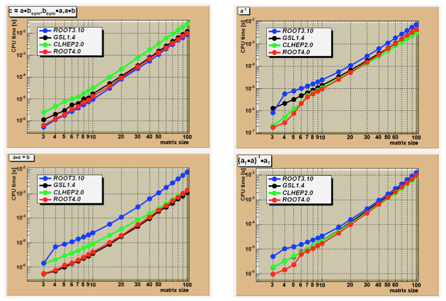
const Bool_t ok = VerifyVectorIdentity(sig,eigenVal,1,1.-e-14);Speed of four matrix operations have been compared between four matrix libraries, GSL CLHEP, ROOT v3.10 and ROOT v4.0. Next figure shows the CPU time for these four operations as a function of the matrix size:
A*B The execution time is measured for the sum of A * Bsym, Bsym* A and A * B. Notice the matrix_size3 dependence of execution time. CLHEP results are hampered by a poor implementation of symmetric matrix multiplications. For instance, for general matrices of size 100x100, the time is 0.015 sec. while A * Bsym takes 0.028 sec and Bsym* A takes 0.059 sec.Both GSL and ROOT v4.0 can be setup to use the hardware-optimized multiplication routines of the BLAS libraries. It was tested on a G4 PowerPC. The improvement becomes clearly visible around sizes of (50x50) were the execution speed improvement of the Altivec processor becomes more significant than the overhead of filling its pipe.
Except for ROOT v3.10, the algorithms are all based on an LUfactorization followed by forward/back-substitution. ROOT v3.10 is using the slower Gaussian elimination method. The numerical accuracy of the CLHEP routine is poor:
up to 6x6 the numerical imprecise Cramer multiplication is hard-coded. For instance, calculating U=H*H-1, where H is a (5x5) Hilbert matrix, results in off-diagonal elements of \(10^{-7}\) instead of the \(10^{-13}\) using an LUaccording to Crout.
scaling protection is non-existent and limits are hard-coded, as a consequence inversion of a Hilbert matrix for sizes>(12x12) fails. In order to gain speed the CLHEP algorithm stores its permutation info of the pivots points in a static array, making multi-threading not possible.
GSL uses LU decomposition without the implicit scaling of Crout. Therefore, its accuracy is not as good. For instance a (10x10) Hilbert matrix has errors 10 times larger than the LU Crout result. In ROOT v4.0, the user can choose between the Invert() and IvertFast() routines, where the latter is using the Cramer algorithm for sizes<7x7. The speed graph shows the result for InvertFast().
A*x=b the execution time is measured for solving the linear equation A*x=b. The same factorizations are used as in the matrix inversion. However, only 1 forward/back-substitution has to be used instead of msize as in the inversion of (msize x msize) matrix. As a consequence the same differences are observed but less amplified. CLHEP shows the same numerical issues as in step the matrix inversion. Since ROOT3.10 has no dedicated equation solver, the solution is calculated through x=A-1*b. This will be slower and numerically not as stable.
\((A^{T}*A)^{-1}*A^{T}\) timing results for calculation of the pseudo inverse of matrix a. The sequence of operations measures the impact of several calls to constructors and destructors in the C++ packages versus a C library like GSL.