class TSPlot: public TObject
Overview
A common method used in High Energy Physics to perform measurements is the maximum Likelihood method, exploiting discriminating variables to disentangle signal from background. The crucial point for such an analysis to be reliable is to use an exhaustive list of sources of events combined with an accurate description of all the Probability Density Functions (PDF).
To assess the validity of the fit, a convincing quality check is to explore further the data sample by examining the distributions of control variables. A control variable can be obtained for instance by removing one of the discriminating variables before performing again the maximum Likelihood fit: this removed variable is a control variable. The expected distribution of this control variable, for signal, is to be compared to the one extracted, for signal, from the data sample. In order to be able to do so, one must be able to unfold from the distribution of the whole data sample.
The TSPlot method allows to reconstruct the distributions for the control variable, independently for each of the various sources of events, without making use of any a priori knowledge on this variable. The aim is thus to use the knowledge available for the discriminating variables to infer the behaviour of the individual sources of events with respect to the control variable.
TSPlot is optimal if the control variable is uncorrelated with the discriminating variables.
A detail description of the formalism itself, called
![]() , is given in [1].
, is given in [1].
The method
The
![]() technique is developped in the above context of a maximum Likelihood method making use of discriminating variables.
technique is developped in the above context of a maximum Likelihood method making use of discriminating variables.
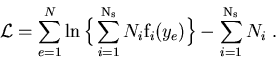
One considers a data sample in which are merged several species of events. These species represent various signal components and background components which all together account for the data sample. The different terms of the log-Likelihood are:
 : the total number of events in the data sample,
-
 : the number of species of events populating the data sample,
 : the number of events expected on the average for the
  species,
-
 : the value of the PDFs of the discriminating variables
  for the
  species and for event
  ,
,
 : the set of control variables which, by definition, do not appear in the expression of the Likelihood function
  .
.
From this expression, after maximization of
where
The distribution of the control variable
The class TSPlot allows to reconstruct the true distribution
![]() of a control variable
of a control variable ![]() for each of the
for each of the
![]() species from the sole knowledge of the PDFs of the discriminating variables
species from the sole knowledge of the PDFs of the discriminating variables ![]() . The plots obtained thanks to the TSPlot class are called
. The plots obtained thanks to the TSPlot class are called
![]() .
.
Some properties and checks
Beside reproducing the true distribution,
![]() bear remarkable properties:
bear remarkable properties:
-
Each -distribution is properly normalized:
-
For any event:
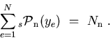
That is to say that, summing up the
 , one recovers the data sample distribution in , and summing up the number of events entering in a
 for a given species, one recovers the yield of the species, as provided by the fit. The property 4 is implemented in the TSPlot class as a check.
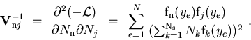
- the sum of the statistical uncertainties per bin
reproduces the statistical uncertainty on the yield , as provided by the fit:
![$\sigma[N_{\rm n}]\equiv\sqrt{\hbox{\bf V}_{{\rm n}{\rm n}}}$](gif/sPlot_img28.png) .
Because of that and since the determination of the yields is optimal
when obtained using a Likelihood fit, one can conclude that the
technique is itself an optimal method to reconstruct distributions of control variables.
.
Because of that and since the determination of the yields is optimal
when obtained using a Likelihood fit, one can conclude that the
technique is itself an optimal method to reconstruct distributions of control variables.
![\begin{displaymath}
\sigma[N_{\rm n}\ _s\tilde{\rm M}_{\rm n}(x) {\delta x}]~=~\sqrt{\sum_{e \subset {\delta x}} ({_s{\cal P}}_{\rm n})^2} ~.
\end{displaymath}](gif/sPlot_img26.png)
Different steps followed by TSPlot
- A maximum Likelihood fit is performed to obtain the yields of the various species.
The fit relies on discriminating variables uncorrelated with a control variable :
the later is therefore totally absent from the fit.
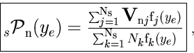
- The weights
 are calculated using Eq. (2) where the covariance matrix is taken from Minuit.
- Histograms of are filled by weighting the events with .
- Error bars per bin are given by Eq. (6).
Illustrations
To illustrate the technique, one considers an example derived from the analysis where
![]() have been first used (charmless B decays). One is dealing with a data
sample in which two species are present: the first is termed signal and
the second background. A maximum Likelihood fit is performed to obtain
the two yields
have been first used (charmless B decays). One is dealing with a data
sample in which two species are present: the first is termed signal and
the second background. A maximum Likelihood fit is performed to obtain
the two yields ![]() and
and ![]() . The fit relies on two discriminating variables collectively denoted
. The fit relies on two discriminating variables collectively denoted ![]() which are chosen within three possible variables denoted
which are chosen within three possible variables denoted ![]() ,
, ![]() and
and ![]() .
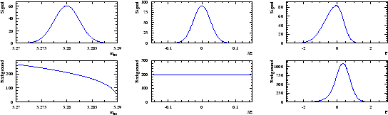
The variable which is not incorporated in
.
The variable which is not incorporated in ![]() is used as the control variable
is used as the control variable ![]() . The six distributions of the three variables are assumed to be the ones depicted in Fig. 1.
. The six distributions of the three variables are assumed to be the ones depicted in Fig. 1.
 |
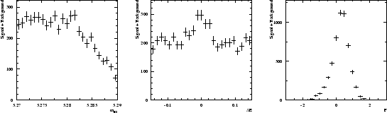
A data sample being built through a Monte Carlo simulation based on the distributions shown in Fig. 1, one obtains the three distributions of Fig. 2. Whereas the distribution of ![]() clearly indicates the presence of the signal, the distribution of
clearly indicates the presence of the signal, the distribution of ![]() and
and ![]() are less obviously populated by signal.
are less obviously populated by signal.
 |
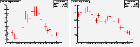
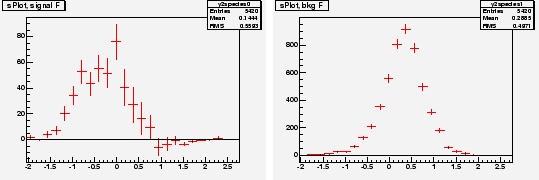
Chosing ![]() and
and ![]() as discriminating variables to determine
as discriminating variables to determine ![]() and
and ![]() through a maximum Likelihood fit, one builds, for the control variable
through a maximum Likelihood fit, one builds, for the control variable ![]() which is unknown to the fit, the two
which is unknown to the fit, the two
![]() for signal and background shown in Fig. 3. One observes that the
for signal and background shown in Fig. 3. One observes that the
![]() for signal reproduces correctly the PDF even where the latter vanishes,
although the error bars remain sizeable. This results from the almost
complete cancellation between positive and negative weights: the sum of
weights is close to zero while the sum of weights squared is not. The
occurence of negative weights occurs through the appearance of the
covariance matrix, and its negative components, in the definition of
Eq. (2).
for signal reproduces correctly the PDF even where the latter vanishes,
although the error bars remain sizeable. This results from the almost
complete cancellation between positive and negative weights: the sum of
weights is close to zero while the sum of weights squared is not. The
occurence of negative weights occurs through the appearance of the
covariance matrix, and its negative components, in the definition of
Eq. (2).
A word of caution is in order with respect to the error bars. Whereas
their sum in quadrature is identical to the statistical uncertainties
of the yields determined by the fit, and if, in addition, they are
asymptotically correct, the error bars should be handled with care for
low statistics and/or for too fine binning. This is because the error
bars do not incorporate two known properties of the PDFs: PDFs are
positive definite and can be non-zero in a given x-bin, even if in the
particular data sample at hand, no event is observed in this bin. The
latter limitation is not specific to
![]() ,
rather it is always present when one is willing to infer the PDF at the
origin of an histogram, when, for some bins, the number of entries does
not guaranty the applicability of the Gaussian regime. In such
situations, a satisfactory practice is to attach allowed ranges to the
histogram to indicate the upper and lower limits of the PDF value which
are consistent with the actual observation, at a given confidence
level.
,
rather it is always present when one is willing to infer the PDF at the
origin of an histogram, when, for some bins, the number of entries does
not guaranty the applicability of the Gaussian regime. In such
situations, a satisfactory practice is to attach allowed ranges to the
histogram to indicate the upper and lower limits of the PDF value which
are consistent with the actual observation, at a given confidence
level.
 |
Chosing ![]() and
and ![]() as discriminating variables to determine
as discriminating variables to determine ![]() and
and ![]() through a maximum Likelihood fit, one builds, for the control variable
through a maximum Likelihood fit, one builds, for the control variable ![]() which is unknown to the fit, the two
which is unknown to the fit, the two
![]() for signal and background shown in Fig. 4. In the
for signal and background shown in Fig. 4. In the
![]() for signal one observes that error bars are the largest in the
for signal one observes that error bars are the largest in the ![]() regions where the background is the largest.
regions where the background is the largest.
 |
The results above can be obtained by running the tutorial TestSPlot.C