IntervalExamples.py File Reference

Detailed Description

Example showing confidence intervals with four techniques.

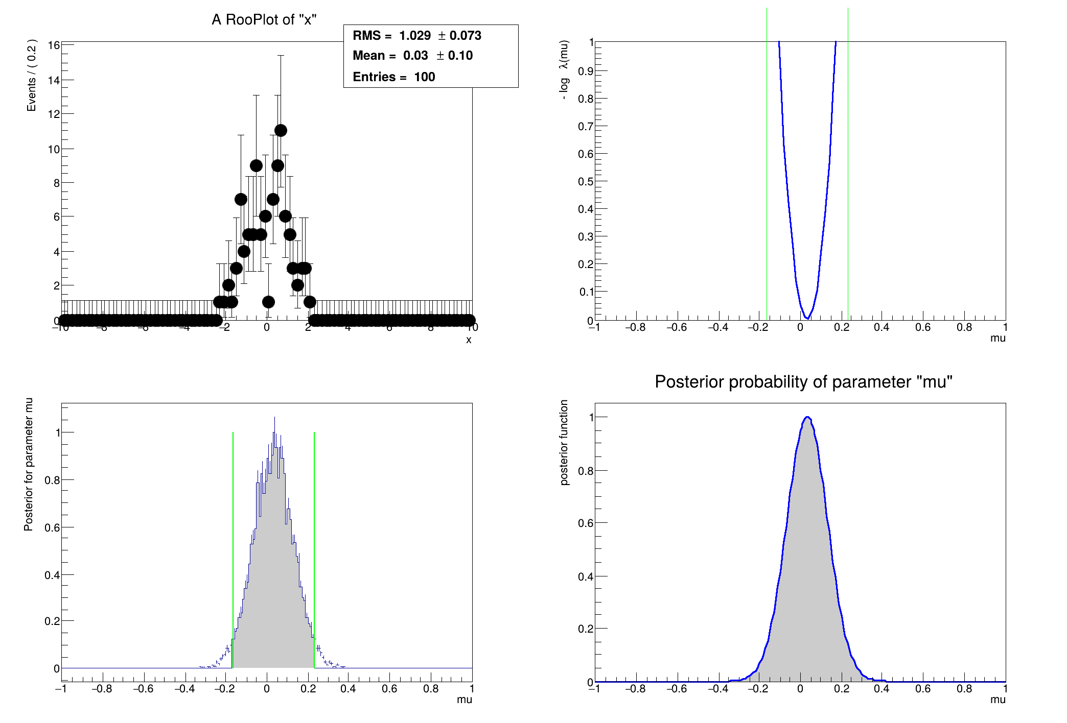
An example that shows confidence intervals with four techniques. The model is a Normal Gaussian G(x|mu,sigma) with 100 samples of x. The answer is known analytically, so this is a good example to validate the RooStats tools.

• expected interval is [-0.162917, 0.229075]
• plc interval is [-0.162917, 0.229075]
• fc interval is [-0.17 , 0.23] // stepsize is 0.01
• bc interval is [-0.162918, 0.229076]
• mcmc interval is [-0.166999, 0.230224]

[#0] WARNING:InputArguments -- The parameter 'sigma' with range [-inf, inf] of the RooGaussian 'normal' exceeds the safe range of (0, inf). Advise to limit its range.
RooDataSet::normalData[x] = 100 entries
[#1] INFO:InputArguments -- The deprecated RooFit::CloneData(1) option passed to createNLL() is ignored.
[#1] INFO:Fitting -- RooAbsPdf::fitTo(normal_over_normal_Int[x]) fixing normalization set for coefficient determination to observables in data
[#1] INFO:Fitting -- using CPU computation library compiled with -mavx2
[#0] PROGRESS:Minimization -- ProfileLikelihoodCalcultor::DoGLobalFit - find MLE 
[#1] INFO:Fitting -- RooAddition::defaultErrorLevel(nll_normal_over_normal_Int[x]_normalData) Summation contains a RooNLLVar, using its error level
[#1] INFO:Minimization -- RooAbsMinimizerFcn::setOptimizeConst: activating const optimization
[#0] PROGRESS:Minimization -- ProfileLikelihoodCalcultor::DoMinimizeNLL - using Minuit2 /  with strategy 1
[#1] INFO:Minimization -- 
  RooFitResult: minimized FCN value: 144.292, estimated distance to minimum: 1.7357e-15
                covariance matrix quality: Full, accurate covariance matrix
                Status : MINIMIZE=0 
 
    Floating Parameter    FinalValue +/-  Error   
  --------------------  --------------------------
                    mu    3.3079e-02 +/-  9.98e-02
 
 
=== Using the following for Example G(x|mu,1) ===
Observables:             RooArgSet:: = (x)
Parameters of Interest:  RooArgSet:: = (mu)
PDF:                     RooGaussian::normal[ x=x mean=mu sigma=sigma ] = 0.999453
 
FeldmanCousins: ntoys per point: adaptive
FeldmanCousins: nEvents per toy will not fluctuate, will always be 100
FeldmanCousins: Model has no nuisance parameters
FeldmanCousins: # points to test = 100
NeymanConstruction: Prog: 1/100 total MC = 78 this test stat = 52.3345
 mu=-0.99 [-inf, 1.44394]  in interval = 0
 
NeymanConstruction: Prog: 2/100 total MC = 78 this test stat = 50.3084
 mu=-0.97 [-inf, 1.79333]  in interval = 0
 
NeymanConstruction: Prog: 3/100 total MC = 78 this test stat = 48.3222
 mu=-0.95 [-inf, 2.15157]  in interval = 0
 
NeymanConstruction: Prog: 4/100 total MC = 78 this test stat = 46.3758
 mu=-0.93 [-inf, 1.35751]  in interval = 0
 
NeymanConstruction: Prog: 5/100 total MC = 78 this test stat = 44.4699
 mu=-0.91 [-inf, 3.34994]  in interval = 0
 
NeymanConstruction: Prog: 6/100 total MC = 78 this test stat = 42.6037
 mu=-0.89 [-inf, 2.51372]  in interval = 0
 
NeymanConstruction: Prog: 7/100 total MC = 78 this test stat = 40.7776
 mu=-0.87 [-inf, 2.23515]  in interval = 0
 
NeymanConstruction: Prog: 8/100 total MC = 78 this test stat = 38.9914
 mu=-0.85 [-inf, 1.58856]  in interval = 0
 
NeymanConstruction: Prog: 9/100 total MC = 78 this test stat = 37.2453
 mu=-0.83 [-inf, 1.815]  in interval = 0
 
NeymanConstruction: Prog: 10/100 total MC = 78 this test stat = 35.5391
 mu=-0.81 [-inf, 2.60213]  in interval = 0
 
NeymanConstruction: Prog: 11/100 total MC = 78 this test stat = 33.873
 mu=-0.79 [-inf, 1.83579]  in interval = 0
 
NeymanConstruction: Prog: 12/100 total MC = 78 this test stat = 32.2468
 mu=-0.77 [-inf, 1.80677]  in interval = 0
 
NeymanConstruction: Prog: 13/100 total MC = 78 this test stat = 30.6606
 mu=-0.75 [-inf, 2.46798]  in interval = 0
 
NeymanConstruction: Prog: 14/100 total MC = 78 this test stat = 29.1145
 mu=-0.73 [-inf, 1.76469]  in interval = 0
 
NeymanConstruction: Prog: 15/100 total MC = 78 this test stat = 27.6083
 mu=-0.71 [-inf, 2.10923]  in interval = 0
 
NeymanConstruction: Prog: 16/100 total MC = 78 this test stat = 26.1422
 mu=-0.69 [-inf, 1.96364]  in interval = 0
 
NeymanConstruction: Prog: 17/100 total MC = 78 this test stat = 24.716
 mu=-0.67 [-inf, 2.46737]  in interval = 0
 
NeymanConstruction: Prog: 18/100 total MC = 78 this test stat = 23.3298
 mu=-0.65 [-inf, 2.22208]  in interval = 0
 
NeymanConstruction: Prog: 19/100 total MC = 78 this test stat = 21.9837
 mu=-0.63 [-inf, 1.92004]  in interval = 0
 
NeymanConstruction: Prog: 20/100 total MC = 78 this test stat = 20.6774
 mu=-0.61 [-inf, 2.09449]  in interval = 0
 
NeymanConstruction: Prog: 21/100 total MC = 78 this test stat = 19.4114
 mu=-0.59 [-inf, 2.82549]  in interval = 0
 
NeymanConstruction: Prog: 22/100 total MC = 78 this test stat = 18.1852
 mu=-0.57 [-inf, 2.44483]  in interval = 0
 
NeymanConstruction: Prog: 23/100 total MC = 78 this test stat = 16.9991
 mu=-0.55 [-inf, 1.47648]  in interval = 0
 
NeymanConstruction: Prog: 24/100 total MC = 78 this test stat = 15.8529
 mu=-0.53 [-inf, 1.64253]  in interval = 0
 
NeymanConstruction: Prog: 25/100 total MC = 78 this test stat = 14.7467
 mu=-0.51 [-inf, 3.23375]  in interval = 0
 
NeymanConstruction: Prog: 26/100 total MC = 78 this test stat = 13.6806
 mu=-0.49 [-inf, 1.36352]  in interval = 0
 
NeymanConstruction: Prog: 27/100 total MC = 78 this test stat = 12.6544
 mu=-0.47 [-inf, 2.24046]  in interval = 0
 
NeymanConstruction: Prog: 28/100 total MC = 78 this test stat = 11.6683
 mu=-0.45 [-inf, 1.99249]  in interval = 0
 
NeymanConstruction: Prog: 29/100 total MC = 78 this test stat = 10.7221
 mu=-0.43 [-inf, 2.54633]  in interval = 0
 
NeymanConstruction: Prog: 30/100 total MC = 78 this test stat = 9.81595
 mu=-0.41 [-inf, 2.19145]  in interval = 0
 
NeymanConstruction: Prog: 31/100 total MC = 78 this test stat = 8.94979
 mu=-0.39 [-inf, 2.25083]  in interval = 0
 
NeymanConstruction: Prog: 32/100 total MC = 78 this test stat = 8.12363
 mu=-0.37 [-inf, 2.63436]  in interval = 0
 
NeymanConstruction: Prog: 33/100 total MC = 78 this test stat = 7.33748
 mu=-0.35 [-inf, 1.7752]  in interval = 0
 
NeymanConstruction: Prog: 34/100 total MC = 78 this test stat = 6.59132
 mu=-0.33 [-inf, 2.63173]  in interval = 0
 
NeymanConstruction: Prog: 35/100 total MC = 78 this test stat = 5.88516
 mu=-0.31 [-inf, 2.2561]  in interval = 0
 
NeymanConstruction: Prog: 36/100 total MC = 78 this test stat = 5.219
 mu=-0.29 [-inf, 2.0388]  in interval = 0
 
NeymanConstruction: Prog: 37/100 total MC = 234 this test stat = 4.59284
 mu=-0.27 [-inf, 1.92574]  in interval = 0
 
NeymanConstruction: Prog: 38/100 total MC = 78 this test stat = 4.00668
 mu=-0.25 [-inf, 2.51905]  in interval = 0
 
NeymanConstruction: Prog: 39/100 total MC = 234 this test stat = 3.46053
 mu=-0.23 [-inf, 2.20004]  in interval = 0
 
NeymanConstruction: Prog: 40/100 total MC = 234 this test stat = 2.95437
 mu=-0.21 [-inf, 1.49924]  in interval = 0
 
NeymanConstruction: Prog: 41/100 total MC = 234 this test stat = 2.48821
 mu=-0.19 [-inf, 1.88454]  in interval = 0
 
NeymanConstruction: Prog: 42/100 total MC = 78 this test stat = 2.06205
 mu=-0.17 [-inf, 2.92073]  in interval = 1
 
NeymanConstruction: Prog: 43/100 total MC = 234 this test stat = 1.6759
 mu=-0.15 [-inf, 2.19199]  in interval = 1
 
NeymanConstruction: Prog: 44/100 total MC = 78 this test stat = 1.32974
 mu=-0.13 [-inf, 1.94832]  in interval = 1
 
NeymanConstruction: Prog: 45/100 total MC = 78 this test stat = 1.02358
 mu=-0.11 [-inf, 2.16863]  in interval = 1
 
NeymanConstruction: Prog: 46/100 total MC = 78 this test stat = 0.757266
 mu=-0.09 [-inf, 1.46141]  in interval = 1
 
NeymanConstruction: Prog: 47/100 total MC = 78 this test stat = 0.531219
 mu=-0.07 [-inf, 4.11006]  in interval = 1
 
NeymanConstruction: Prog: 48/100 total MC = 78 this test stat = 0.345097
 mu=-0.05 [-inf, 2.11338]  in interval = 1
 
NeymanConstruction: Prog: 49/100 total MC = 78 this test stat = 0.198947
 mu=-0.03 [-inf, 2.38127]  in interval = 1
 
NeymanConstruction: Prog: 50/100 total MC = 78 this test stat = 0.09279
 mu=-0.01 [-inf, 3.0189]  in interval = 1
 
NeymanConstruction: Prog: 51/100 total MC = 78 this test stat = 0.026632
 mu=0.01 [-inf, 2.23423]  in interval = 1
 
NeymanConstruction: Prog: 52/100 total MC = 78 this test stat = 0.000474009
 mu=0.03 [-inf, 2.54313]  in interval = 1
 
NeymanConstruction: Prog: 53/100 total MC = 78 this test stat = 0.014316
 mu=0.05 [-inf, 1.52484]  in interval = 1
 
NeymanConstruction: Prog: 54/100 total MC = 78 this test stat = 0.0681571
 mu=0.07 [-inf, 2.72021]  in interval = 1
 
NeymanConstruction: Prog: 55/100 total MC = 78 this test stat = 0.161992
 mu=0.09 [-inf, 3.26474]  in interval = 1
 
NeymanConstruction: Prog: 56/100 total MC = 78 this test stat = 0.2958
 mu=0.11 [-inf, 2.81134]  in interval = 1
 
NeymanConstruction: Prog: 57/100 total MC = 78 this test stat = 0.469534
 mu=0.13 [-inf, 2.59127]  in interval = 1
 
NeymanConstruction: Prog: 58/100 total MC = 78 this test stat = 0.683526
 mu=0.15 [-inf, 2.60194]  in interval = 1
 
NeymanConstruction: Prog: 59/100 total MC = 78 this test stat = 0.937368
 mu=0.17 [-inf, 1.94974]  in interval = 1
 
NeymanConstruction: Prog: 60/100 total MC = 78 this test stat = 1.23121
 mu=0.19 [-inf, 1.73838]  in interval = 1
 
NeymanConstruction: Prog: 61/100 total MC = 702 this test stat = 1.56505
 mu=0.21 [-inf, 1.73023]  in interval = 1
 
NeymanConstruction: Prog: 62/100 total MC = 78 this test stat = 1.93888
 mu=0.23 [-inf, 3.06401]  in interval = 1
 
NeymanConstruction: Prog: 63/100 total MC = 234 this test stat = 2.35273
 mu=0.25 [-inf, 1.63166]  in interval = 0
 
NeymanConstruction: Prog: 64/100 total MC = 234 this test stat = 2.80658
 mu=0.27 [-inf, 1.83441]  in interval = 0
 
NeymanConstruction: Prog: 65/100 total MC = 234 this test stat = 3.30042
 mu=0.29 [-inf, 2.06725]  in interval = 0
 
NeymanConstruction: Prog: 66/100 total MC = 78 this test stat = 3.83426
 mu=0.31 [-inf, 2.10484]  in interval = 0
 
NeymanConstruction: Prog: 67/100 total MC = 78 this test stat = 4.4081
 mu=0.33 [-inf, 2.1714]  in interval = 0
 
NeymanConstruction: Prog: 68/100 total MC = 78 this test stat = 5.02195
 mu=0.35 [-inf, 2.77418]  in interval = 0
 
NeymanConstruction: Prog: 69/100 total MC = 78 this test stat = 5.67579
 mu=0.37 [-inf, 2.39797]  in interval = 0
 
NeymanConstruction: Prog: 70/100 total MC = 78 this test stat = 6.36963
 mu=0.39 [-inf, 1.83585]  in interval = 0
 
NeymanConstruction: Prog: 71/100 total MC = 78 this test stat = 7.10347
 mu=0.41 [-inf, 1.92776]  in interval = 0
 
NeymanConstruction: Prog: 72/100 total MC = 78 this test stat = 7.87731
 mu=0.43 [-inf, 1.62512]  in interval = 0
 
NeymanConstruction: Prog: 73/100 total MC = 78 this test stat = 8.69116
 mu=0.45 [-inf, 1.5721]  in interval = 0
 
NeymanConstruction: Prog: 74/100 total MC = 78 this test stat = 9.545
 mu=0.47 [-inf, 1.9811]  in interval = 0
 
NeymanConstruction: Prog: 75/100 total MC = 78 this test stat = 10.4388
 mu=0.49 [-inf, 3.71619]  in interval = 0
 
NeymanConstruction: Prog: 76/100 total MC = 78 this test stat = 11.3727
 mu=0.51 [-inf, 2.09734]  in interval = 0
 
NeymanConstruction: Prog: 77/100 total MC = 78 this test stat = 12.3465
 mu=0.53 [-inf, 1.61789]  in interval = 0
 
NeymanConstruction: Prog: 78/100 total MC = 78 this test stat = 13.3604
 mu=0.55 [-inf, 1.75937]  in interval = 0
 
NeymanConstruction: Prog: 79/100 total MC = 78 this test stat = 14.4142
 mu=0.57 [-inf, 2.16051]  in interval = 0
 
NeymanConstruction: Prog: 80/100 total MC = 78 this test stat = 15.5081
 mu=0.59 [-inf, 2.48971]  in interval = 0
 
NeymanConstruction: Prog: 81/100 total MC = 78 this test stat = 16.6419
 mu=0.61 [-inf, 2.15114]  in interval = 0
 
NeymanConstruction: Prog: 82/100 total MC = 78 this test stat = 17.8157
 mu=0.63 [-inf, 2.63832]  in interval = 0
 
NeymanConstruction: Prog: 83/100 total MC = 78 this test stat = 19.0296
 mu=0.65 [-inf, 2.12006]  in interval = 0
 
NeymanConstruction: Prog: 84/100 total MC = 78 this test stat = 20.2834
 mu=0.67 [-inf, 1.70414]  in interval = 0
 
NeymanConstruction: Prog: 85/100 total MC = 78 this test stat = 21.5773
 mu=0.69 [-inf, 2.54958]  in interval = 0
 
NeymanConstruction: Prog: 86/100 total MC = 78 this test stat = 22.9111
 mu=0.71 [-inf, 2.27992]  in interval = 0
 
NeymanConstruction: Prog: 87/100 total MC = 78 this test stat = 24.2849
 mu=0.73 [-inf, 2.99068]  in interval = 0
 
NeymanConstruction: Prog: 88/100 total MC = 78 this test stat = 25.6988
 mu=0.75 [-inf, 1.60655]  in interval = 0
 
NeymanConstruction: Prog: 89/100 total MC = 78 this test stat = 27.1526
 mu=0.77 [-inf, 1.61728]  in interval = 0
 
NeymanConstruction: Prog: 90/100 total MC = 78 this test stat = 28.6465
 mu=0.79 [-inf, 1.92571]  in interval = 0
 
NeymanConstruction: Prog: 91/100 total MC = 78 this test stat = 30.1803
 mu=0.81 [-inf, 1.69221]  in interval = 0
 
NeymanConstruction: Prog: 92/100 total MC = 78 this test stat = 31.7542
 mu=0.83 [-inf, 3.26227]  in interval = 0
 
NeymanConstruction: Prog: 93/100 total MC = 78 this test stat = 33.368
 mu=0.85 [-inf, 1.75583]  in interval = 0
 
NeymanConstruction: Prog: 94/100 total MC = 78 this test stat = 35.0218
 mu=0.87 [-inf, 2.54103]  in interval = 0
 
NeymanConstruction: Prog: 95/100 total MC = 78 this test stat = 36.7157
 mu=0.89 [-inf, 2.267]  in interval = 0
 
NeymanConstruction: Prog: 96/100 total MC = 78 this test stat = 38.4495
 mu=0.91 [-inf, 2.31167]  in interval = 0
 
NeymanConstruction: Prog: 97/100 total MC = 78 this test stat = 40.2234
 mu=0.93 [-inf, 2.24794]  in interval = 0
 
NeymanConstruction: Prog: 98/100 total MC = 78 this test stat = 42.0372
 mu=0.95 [-inf, 1.29779]  in interval = 0
 
NeymanConstruction: Prog: 99/100 total MC = 78 this test stat = 43.891
 mu=0.97 [-inf, 2.00008]  in interval = 0
 
NeymanConstruction: Prog: 100/100 total MC = 78 this test stat = 45.7849
 mu=0.99 [-inf, 1.56062]  in interval = 0
 
[#1] INFO:Eval -- 21 points in interval
[#1] INFO:Fitting -- RooAbsPdf::fitTo(normal_over_normal_Int[x]) fixing normalization set for coefficient determination to observables in data
[#1] INFO:Eval -- BayesianCalculator::GetPosteriorFunction :  nll value 190.077 poi value = 0.99
[#1] INFO:Eval -- BayesianCalculator::GetPosteriorFunction : minimum of NLL vs POI for POI =  0.033079 min NLL = 144.292
[#1] INFO:Minimization --  Including the following constraint terms in minimization: (prior)
[#1] INFO:Minimization -- The following global observables have been defined and their values are taken from the model: ()
[#1] INFO:Fitting -- RooAbsPdf::fitTo(product_normal_prior) fixing normalization set for coefficient determination to observables in data
[#1] INFO:Eval -- BayesianCalculator: Compute interval using RooFit:  posteriorPdf + createCdf + RooBrentRootFinder 
[#1] INFO:Eval -- BayesianCalculator::GetInterval - found a valid interval : [-0.95 , 0.95 ]
[#1] INFO:Minimization --  Including the following constraint terms in minimization: (prior)
[#1] INFO:Minimization -- The following global observables have been defined and their values are taken from the model: ()
[#1] INFO:Fitting -- RooAbsPdf::fitTo(product_normal_prior) fixing normalization set for coefficient determination to observables in data
Metropolis-Hastings progress: ....................................................................................................
[#1] INFO:Eval -- Proposal acceptance rate: 16.013%
[#1] INFO:Eval -- Number of steps in chain: 16013
.
[#1] INFO:Minimization -- RooProfileLL::evaluate(RooEvaluatorWrapper_Profile[mu]) Creating instance of MINUIT
[#1] INFO:Fitting -- RooAddition::defaultErrorLevel(nll_normal_over_normal_Int[x]_normalData) Summation contains a RooNLLVar, using its error level
[#1] INFO:Minimization -- RooProfileLL::evaluate(RooEvaluatorWrapper_Profile[mu]) determining minimum likelihood for current configurations w.r.t all observable
[#0] ERROR:InputArguments -- RooArgSet::checkForDup: ERROR argument with name mu is already in this set
[#1] INFO:Minimization -- RooProfileLL::evaluate(RooEvaluatorWrapper_Profile[mu]) minimum found at (mu=0.033079)
..........................................................................................................................................................................................................Real time 0:00:05, CP time 5.360
expected interval is [-0.1629174085659928, 0.22907538834201802]
plc interval is [-0.16291740856540754, 0.22907538834167748]
fc interval is [-0.16999999999999993, 0.22999999999999998]
bc interval is [-0.95, 0.9500000000000002]
mc interval is [-0.1669991221278906, 0.23022447898983955]
is mu=0 in the interval?  True

 
import ROOT
 
# Time this macro
t = ROOT.TStopwatch()
t.Start()
 
# set RooFit random seed for reproducible results
ROOT.RooRandom.randomGenerator().SetSeed(3001)
 
# make a simple model via the workspace factory
wspace = ROOT.RooWorkspace()
wspace.factory("Gaussian::normal(x[-10,10],mu[-1,1],sigma[1])")
wspace.defineSet("poi", "mu")
wspace.defineSet("obs", "x")
 
# specify components of model for statistical tools
modelConfig = ROOT.RooStats.ModelConfig("Example G(x|mu,1)")
modelConfig.SetWorkspace(wspace)
modelConfig.SetPdf(wspace["normal"])
modelConfig.SetParametersOfInterest(wspace.set("poi"))
modelConfig.SetObservables(wspace.set("obs"))
 
# create a toy dataset
data = wspace["normal"].generate(wspace.set("obs"), 100)
data.Print()
 
# for convenience later on
x = wspace["x"]
mu = wspace["mu"]
 
# set confidence level
confidenceLevel = 0.95
 
# example use profile likelihood calculator
plc = ROOT.RooStats.ProfileLikelihoodCalculator(data, modelConfig)
plc.SetConfidenceLevel(confidenceLevel)
plInt = plc.GetInterval()
 
# example use of Feldman-Cousins
fc = ROOT.RooStats.FeldmanCousins(data, modelConfig)
fc.SetConfidenceLevel(confidenceLevel)
fc.SetNBins(100)  # number of points to test per parameter
fc.UseAdaptiveSampling(True)  # make it go faster
 
# Here, we consider only ensembles with 100 events
# The PDF could be extended and this could be removed
fc.FluctuateNumDataEntries(False)
 
interval = fc.GetInterval()
 
# example use of BayesianCalculator
# now we also need to specify a prior in the ModelConfig
wspace.factory("Uniform::prior(mu)")
modelConfig.SetPriorPdf(wspace["prior"])
 
# example usage of BayesianCalculator
bc = ROOT.RooStats.BayesianCalculator(data, modelConfig)
bc.SetConfidenceLevel(confidenceLevel)
bcInt = bc.GetInterval()
 
# example use of MCMCInterval
mc = ROOT.RooStats.MCMCCalculator(data, modelConfig)
mc.SetConfidenceLevel(confidenceLevel)
# special options
mc.SetNumBins(200)  # bins used internally for representing posterior
mc.SetNumBurnInSteps(500)  # first N steps to be ignored as burn-in
mc.SetNumIters(100000)  # how long to run chain
mc.SetLeftSideTailFraction(0.5)  # for central interval
mcInt = mc.GetInterval()
 
# for this example we know the expected intervals
expectedLL = data.mean(x) + ROOT.Math.normal_quantile((1 - confidenceLevel) / 2, 1) / ROOT.sqrt(data.numEntries())
expectedUL = data.mean(x) + ROOT.Math.normal_quantile_c((1 - confidenceLevel) / 2, 1) / ROOT.sqrt(data.numEntries())
 
# Use the intervals
print("expected interval is [{}, {}]".format(expectedLL, expectedUL))
print("plc interval is [{}, {}]".format(plInt.LowerLimit(mu), plInt.UpperLimit(mu)))
print("fc interval is [{}, {}]".format(interval.LowerLimit(mu), interval.UpperLimit(mu)))
print("bc interval is [{}, {}]".format(bcInt.LowerLimit(), bcInt.UpperLimit()))
print("mc interval is [{}, {}]".format(mcInt.LowerLimit(mu), mcInt.UpperLimit(mu)))
mu.setVal(0)
print("is mu=0 in the interval? ", plInt.IsInInterval({mu}))
 
# make a reasonable style
ROOT.gStyle.SetCanvasColor(0)
ROOT.gStyle.SetCanvasBorderMode(0)
ROOT.gStyle.SetPadBorderMode(0)
ROOT.gStyle.SetPadColor(0)
ROOT.gStyle.SetCanvasColor(0)
ROOT.gStyle.SetTitleFillColor(0)
ROOT.gStyle.SetFillColor(0)
ROOT.gStyle.SetFrameFillColor(0)
ROOT.gStyle.SetStatColor(0)
 
# some plots
canvas = ROOT.TCanvas("canvas")
canvas.Divide(2, 2)
 
# plot the data
canvas.cd(1)
frame = x.frame()
data.plotOn(frame)
data.statOn(frame)
frame.Draw()
 
# plot the profile likelihood
canvas.cd(2)
plot = ROOT.RooStats.LikelihoodIntervalPlot(plInt)
plot.Draw()
 
# plot the MCMC interval
canvas.cd(3)
mcPlot = ROOT.RooStats.MCMCIntervalPlot(mcInt)
mcPlot.SetLineColor(ROOT.kGreen)
mcPlot.SetLineWidth(2)
mcPlot.Draw()
 
canvas.cd(4)
bcPlot = bc.GetPosteriorPlot()
bcPlot.Draw()
 
canvas.Update()
 
t.Stop()
t.Print()
 
canvas.SaveAs("IntervalExamples.png")
 
# TODO: The BayesianCalculator and MCMCCalculator have to be destructed first.
# Otherwise, we can get segmentation faults depending on the destruction order,
# which is random in Python. Probably the issue is that some object has a
# non-owning pointer to another object, which it uses in its destructor. This
# should be fixed either in the design of RooStats in C++, or with
# phythonizations.
del bc
del mc

Date

July 2022

Authors

Artem Busorgin, Kyle Cranmer (C++ version)

Definition in file IntervalExamples.py.