TGraphPainter Class Reference

The graph painter class.

Implements all graphs' drawing's options.

• Introduction
• Graphs' plotting options
• Exclusion graphs
• Graphs with error bars
  • TGraphErrors
  • TGraphAsymmErrors
  • TGraphBentErrors
• TGraphPolar options
• Colors automatically picked in palette
• Reverse graphs' axis
• Graphs in logarithmic scale
• Highlight mode for graph

Introduction

Graphs are drawn via the painter TGraphPainter class. This class implements techniques needed to display the various kind of graphs i.e.: TGraph, TGraphErrors, TGraphBentErrors and TGraphAsymmErrors.

To draw a graph graph it's enough to do:

graph->Draw("AL");

The option AL in the Draw() method means:

1. The axis should be drawn (option A),

2. The graph should be drawn as a simple line (option L).

   By default a graph is drawn in the current pad in the current coordinate system. To define a suitable coordinate system and draw the axis the option A must be specified.

TGraphPainter offers many options to paint the various kind of graphs.

It is separated from the graph classes so that one can have graphs without the graphics overhead, for example in a batch program.

When a displayed graph is modified, there is no need to call Draw() again; the image will be refreshed the next time the pad will be updated. A pad is updated after one of these three actions:

1. a carriage return on the ROOT command line,
2. a click inside the pad,
3. a call to TPad::Update.

Graphs' plotting options

Graphs can be drawn with the following options:

Option	Description
"A"	Axis are drawn around the graph
"I"	Combine with option 'A' it draws invisible axis
"L"	A simple polyline is drawn
"F"	A fill area is drawn ('CF' draw a smoothed fill area)
"C"	A smooth Curve is drawn
"*"	A Star is plotted at each point
"P"	The current marker is plotted at each point
"B"	A Bar chart is drawn
"1"	When a graph is drawn as a bar chart, this option makes the bars start from the bottom of the pad. By default they start at 0.
"X+"	The X-axis is drawn on the top side of the plot.
"Y+"	The Y-axis is drawn on the right side of the plot.
"PFC"	Palette Fill Color: graph's fill color is taken in the current palette.
"PLC"	Palette Line Color: graph's line color is taken in the current palette.
"PMC"	Palette Marker Color: graph's marker color is taken in the current palette.
"RX"	Reverse the X axis.
"RY"	Reverse the Y axis.

Drawing options can be combined. In the following example the graph is drawn as a smooth curve (option "C") with markers (option "P") and with axes (option "A").

{
   auto c1 = new TCanvas("c1","c1",200,10,600,400);
 
   c1->SetFillColor(42);
   c1->SetGrid();
 
   const Int_t n = 20;
   Double_t x[n], y[n];
   for (Int_t i=0;i<n;i++) {
      x[i] = i*0.1;
      y[i] = 10*sin(x[i]+0.2);
   }
   gr = new TGraph(n,x,y);
   gr->SetLineColor(2);
   gr->SetLineWidth(4);
   gr->SetMarkerColor(4);
   gr->SetMarkerSize(1.5);
   gr->SetMarkerStyle(21);
   gr->SetTitle("Option ACP example");
   gr->GetXaxis()->SetTitle("X title");
   gr->GetYaxis()->SetTitle("Y title");
   gr->Draw("ACP");
 
   // TCanvas::Update() draws the frame, after which one can change it
   c1->Update();
   c1->GetFrame()->SetFillColor(21);
   c1->GetFrame()->SetBorderSize(12);
   c1->Modified();
}

The following macro shows the option "B" usage. It can be combined with the option "1".

{
   auto c47 = new TCanvas("c47","c47",200,10,600,400);
   c47->Divide(1,2);
   const Int_t n = 20;
   Double_t x[n], y[n];
   for (Int_t i=0;i<n;i++) {
      x[i] = i*0.1;
      y[i] = 10*sin(x[i]+0.2)-6;
   }
   gr = new TGraph(n,x,y);
   gr->SetFillColor(38);
   c47->cd(1); gr->Draw("AB");
   c47->cd(2); gr->Draw("AB1");
}

Exclusion graphs

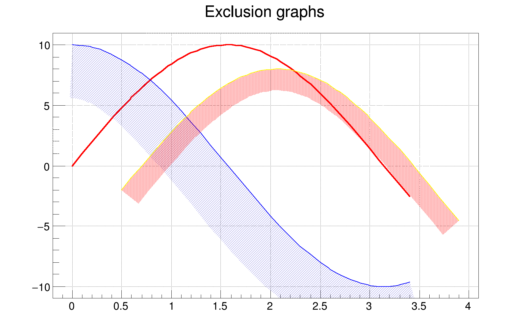
When a graph is painted with the option C or L it is possible to draw a filled area on one side of the line. This is useful to show exclusion zones.

This drawing mode is activated when the absolute value of the graph line width (set by SetLineWidth()) is greater than 99. In that case the line width number is interpreted as:

100*ff+ll = ffll

• The two digits number ll represent the normal line width
• The two digits number ff represent the filled area width.
• The sign of "ffll" allows to flip the filled area from one side of the line to the other.

The current fill area attributes are used to draw the hatched zone.

 
TCanvas *exclusiongraph() {
   TCanvas *c1 = new TCanvas("c1","Exclusion graphs examples",200,10,600,400);
   c1->SetGrid();
 
   TMultiGraph *mg = new TMultiGraph();
   mg->SetTitle("Exclusion graphs");
 
   const Int_t n = 35;
   Double_t xvalues1[n], xvalues2[n], xvalues3[n], yvalues1[n], yvalues2[n], yvalues3[n];
   for (Int_t i=0;i<n;i++) {
     xvalues1[i]  = i*0.1;
     xvalues2[i]  = xvalues1[i];
     xvalues3[i]  = xvalues1[i]+.5;
     yvalues1[i] = 10*sin(xvalues1[i]);
     yvalues2[i] = 10*cos(xvalues1[i]);
     yvalues3[i] = 10*sin(xvalues1[i])-2;
   }
 
   TGraph *gr1 = new TGraph(n,xvalues1,yvalues1);
   gr1->SetLineColor(2);
   gr1->SetLineWidth(1504);
   gr1->SetFillStyle(3005);
 
   TGraph *gr2 = new TGraph(n,xvalues2,yvalues2);
   gr2->SetLineColor(4);
   gr2->SetLineWidth(-2002);
   gr2->SetFillStyle(3004);
   gr2->SetFillColor(9);
 
   TGraph *gr3 = new TGraph(n,xvalues3,yvalues3);
   gr3->SetLineColor(5);
   gr3->SetLineWidth(-802);
   gr3->SetFillStyle(3002);
   gr3->SetFillColor(2);
 
   mg->Add(gr1);
   mg->Add(gr2);
   mg->Add(gr3);
   mg->Draw("AC");
 
   return c1;
}

Graphs with error bars

Three classes are available to handle graphs with error bars: TGraphErrors, TGraphAsymmErrors and TGraphBentErrors. The following drawing options are specific to graphs with error bars:

Option	Description
"Z"	Do not draw small horizontal and vertical lines the end of the error bars. Without "Z", the default is to draw these.
">"	An arrow is drawn at the end of the error bars. The size of the arrow is set to 2/3 of the marker size.
"|>"	A filled arrow is drawn at the end of the error bars. The size of the arrow is set to 2/3 of the marker size.
"X"	Do not draw error bars. By default, graph classes that have errors are drawn with the errors (TGraph itself has no errors, and so this option has no effect.)
"||"	Draw only the small vertical/horizontal lines at the ends of the error bars, without drawing the bars themselves. This option is interesting to superimpose statistical-only errors on top of a graph with statistical+systematic errors.
"[]"	Does the same as option "||" except that it draws additional marks at the ends of the small vertical/horizontal lines. It makes plots less ambiguous in case several graphs are drawn on the same picture.
"0"	By default, when a data point is outside the visible range along the Y axis, the error bars are not drawn. This option forces error bars' drawing for the data points outside the visible range along the Y axis (see example below).
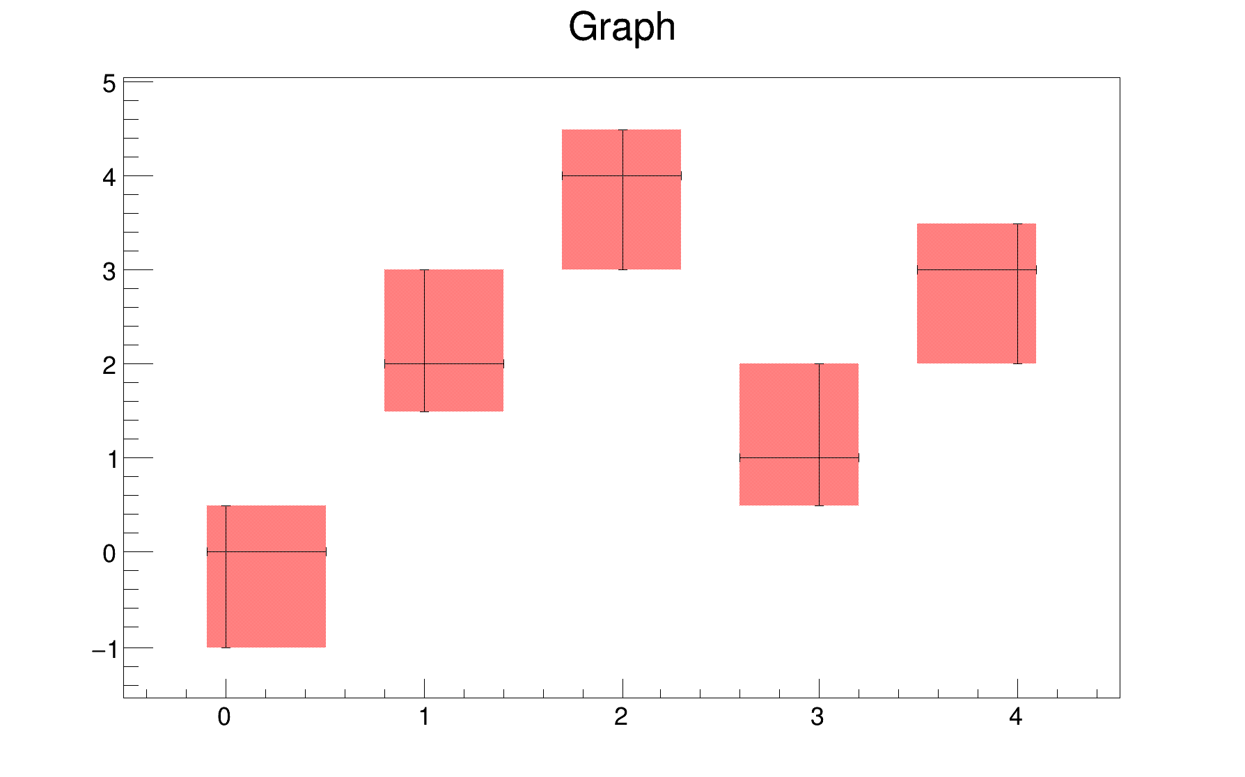
"2"	Error rectangles are drawn.
"3"	A filled area is drawn through the end points of the vertical error bars.
"4"	A smoothed filled area is drawn through the end points of the vertical error bars.
"5"	Error rectangles are drawn like option "2". In addition the contour line around the boxes is drawn. This can be useful when boxes' fill colors are very light or in gray scale mode.

gStyle->SetErrorX(dx) controls the size of the error along x. dx = 0 removes the error along x.

gStyle->SetEndErrorSize(np) controls the size of the lines at the end of the error bars (when option 1 is used). By default np=1. (np represents the number of pixels).

TGraphErrors

A TGraphErrors is a TGraph with error bars. The errors are defined along X and Y and are symmetric: The left and right errors are the same along X and the bottom and up errors are the same along Y.

{
   auto c4 = new TCanvas("c4","c4",200,10,600,400);
   double x[] = {0, 1, 2, 3, 4};
   double y[] = {0, 2, 4, 1, 3};
   double ex[] = {0.1, 0.2, 0.3, 0.4, 0.5};
   double ey[] = {1, 0.5, 1, 0.5, 1};
   TGraphErrors* ge = new TGraphErrors(5, x, y, ex, ey);
   ge->Draw("ap");
}

The option "0" shows the error bars for data points outside range.

{
   auto c48 = new TCanvas("c48","c48",200,10,600,400);
   float x[]     = {1,2,3};
   float err_x[] = {0,0,0};
   float err_y[] = {5,5,5};
   float y[]     = {1,4,9};
   TGraphErrors tg(3,x,y,err_x,err_y);
   c48->Divide(2,1);
   c48->cd(1); gPad->DrawFrame(0,0,4,8); tg.Draw("PC");
   c48->cd(2); gPad->DrawFrame(0,0,4,8); tg.Draw("0PC");
}

The option "3" shows the errors as a band.

{
   auto c41 = new TCanvas("c41","c41",200,10,600,400);
   double x[] = {0, 1, 2, 3, 4};
   double y[] = {0, 2, 4, 1, 3};
   double ex[] = {0.1, 0.2, 0.3, 0.4, 0.5};
   double ey[] = {1, 0.5, 1, 0.5, 1};
   TGraphErrors* ge = new TGraphErrors(5, x, y, ex, ey);
   ge->SetFillColor(4);
   ge->SetFillStyle(3010);
   ge->Draw("a3");
}

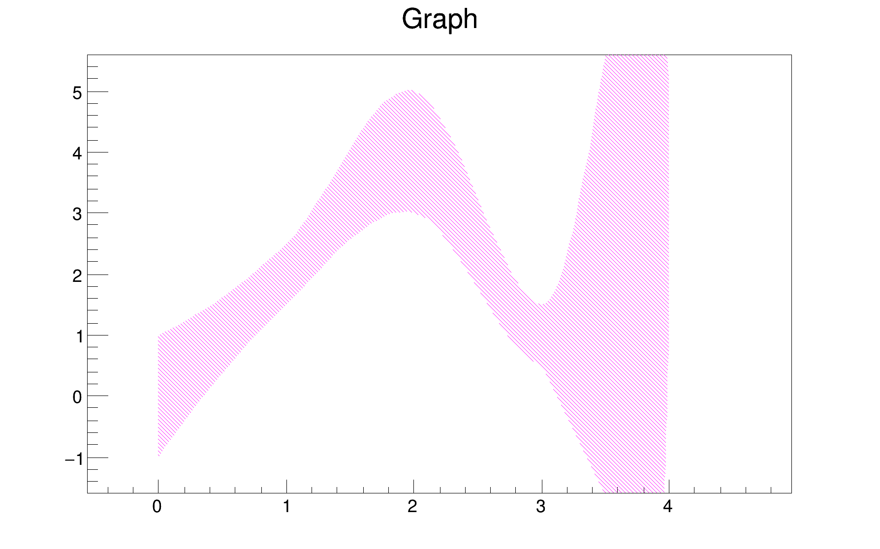
The option "4" is similar to the option "3" except that the band is smoothed. As the following picture shows, this option should be used carefully because the smoothing algorithm may show some (huge) "bouncing" effects. In some cases it looks nicer than option "3" (because it is smooth) but it can be misleading.

{
   auto c42 = new TCanvas("c42","c42",200,10,600,400);
   double x[] = {0, 1, 2, 3, 4};
   double y[] = {0, 2, 4, 1, 3};
   double ex[] = {0.1, 0.2, 0.3, 0.4, 0.5};
   double ey[] = {1, 0.5, 1, 0.5, 1};
   TGraphErrors* ge = new TGraphErrors(5, x, y, ex, ey);
   ge->SetFillColor(6);
   ge->SetFillStyle(3005);
   ge->Draw("a4");
}

The following example shows how the option "[]" can be used to superimpose systematic errors on top of a graph with statistical errors.

{
   auto c43 = new TCanvas("c43","c43",200,10,600,400);
   c43->DrawFrame(0., -0.5, 6., 2);
 
   double x[5]    = {1, 2, 3, 4, 5};
   double zero[5] = {0, 0, 0, 0, 0};
 
   // data set (1) with stat and sys errors
   double py1[5]      = {1.2, 1.15, 1.19, 0.9, 1.4};
   double ey_stat1[5] = {0.2, 0.18, 0.17, 0.2, 0.4};
   double ey_sys1[5]  = {0.5, 0.71, 0.76, 0.5, 0.45};
 
   // data set (2) with stat and sys errors
   double y2[5]       = {0.25, 0.18, 0.29, 0.2, 0.21};
   double ey_stat2[5] = {0.2, 0.18, 0.17, 0.2, 0.4};
   double ey_sys2[5]  = {0.63, 0.19, 0.7, 0.2, 0.7};
 
   // Now draw data set (1)
 
   // We first have to draw it only with the stat errors
   TGraphErrors *graph1 = new TGraphErrors(5, x, py1, zero, ey_stat1);
   graph1->SetMarkerStyle(20);
   graph1->Draw("P");
 
   // Now we have to somehow depict the sys errors
 
   TGraphErrors *graph1_sys = new TGraphErrors(5, x, py1, zero, ey_sys1);
   graph1_sys->Draw("[]");
 
   // Now draw data set (2)
 
   // We first have to draw it only with the stat errors
   TGraphErrors *graph2 = new TGraphErrors(5, x, y2, zero, ey_stat2);
   graph2->SetMarkerStyle(24);
   graph2->Draw("P");
 
   // Now we have to somehow depict the sys errors
 
   TGraphErrors *graph2_sys = new TGraphErrors(5, x, y2, zero, ey_sys2);
   graph2_sys->Draw("[]");
}

TGraphAsymmErrors

A TGraphAsymmErrors is like a TGraphErrors but the errors defined along X and Y are not symmetric: The left and right errors are different along X and the bottom and up errors are different along Y.

{
   auto c44 = new TCanvas("c44","c44",200,10,600,400);
   double ax[] = {0, 1, 2, 3, 4};
   double ay[] = {0, 2, 4, 1, 3};
   double aexl[] = {0.1, 0.2, 0.3, 0.4, 0.5};
   double aexh[] = {0.5, 0.4, 0.3, 0.2, 0.1};
   double aeyl[] = {1, 0.5, 1, 0.5, 1};
   double aeyh[] = {0.5, 1, 0.5, 1, 0.5};
   TGraphAsymmErrors* gae = new TGraphAsymmErrors(5, ax, ay, aexl, aexh, aeyl, aeyh);
   gae->SetFillColor(2);
   gae->SetFillStyle(3001);
   gae->Draw("a2");
   gae->Draw("p");
}

TGraphBentErrors

A TGraphBentErrors is like a TGraphAsymmErrors. An extra parameter allows to bend the error bars to better see them when several graphs are drawn on the same plot.

{
   auto c45 = new TCanvas("c45","c45",200,10,600,400);
   const Int_t n = 10;
   Double_t x[n]  = {-0.22, 0.05, 0.25, 0.35, 0.5, 0.61,0.7,0.85,0.89,0.95};
   Double_t y[n]  = {1,2.9,5.6,7.4,9,9.6,8.7,6.3,4.5,1};
   Double_t exl[n] = {.05,.1,.07,.07,.04,.05,.06,.07,.08,.05};
   Double_t eyl[n] = {.8,.7,.6,.5,.4,.4,.5,.6,.7,.8};
   Double_t exh[n] = {.02,.08,.05,.05,.03,.03,.04,.05,.06,.03};
   Double_t eyh[n] = {.6,.5,.4,.3,.2,.2,.3,.4,.5,.6};
   Double_t exld[n] = {.0,.0,.0,.0,.0,.0,.0,.0,.0,.0};
   Double_t eyld[n] = {.0,.0,.05,.0,.0,.0,.0,.0,.0,.0};
   Double_t exhd[n] = {.0,.0,.0,.0,.0,.0,.0,.0,.0,.0};
   Double_t eyhd[n] = {.0,.0,.0,.0,.0,.0,.0,.0,.05,.0};
   TGraphBentErrors *gr = new TGraphBentErrors(n,x,y,exl,exh,eyl,eyh,exld,exhd,eyld,eyhd);
   gr->SetTitle("TGraphBentErrors Example");
   gr->SetMarkerColor(4);
   gr->SetMarkerStyle(21);
   gr->Draw("ALP");
}

TGraphPolar options

The drawing options for the polar graphs are the following:

Option	Description
"O"	Polar labels are drawn orthogonally to the polargram radius.
"P"	Polymarker are drawn at each point position.
"E"	Draw error bars.
"F"	Draw fill area (closed polygon).
"A"	Force axis redrawing even if a polargram already exists.
"N"	Disable the display of the polar labels.

{
   auto c46 = new TCanvas("c46","c46",500,500);
   TGraphPolar * grP1 = new TGraphPolar();
   grP1->SetTitle("TGraphPolar example");
 
   grP1->SetPoint(0, (1*TMath::Pi())/4., 0.05);
   grP1->SetPoint(1, (2*TMath::Pi())/4., 0.10);
   grP1->SetPoint(2, (3*TMath::Pi())/4., 0.15);
   grP1->SetPoint(3, (4*TMath::Pi())/4., 0.20);
   grP1->SetPoint(4, (5*TMath::Pi())/4., 0.25);
   grP1->SetPoint(5, (6*TMath::Pi())/4., 0.30);
   grP1->SetPoint(6, (7*TMath::Pi())/4., 0.35);
   grP1->SetPoint(7, (8*TMath::Pi())/4., 0.40);
 
   grP1->SetMarkerStyle(20);
   grP1->SetMarkerSize(1.);
   grP1->SetMarkerColor(4);
   grP1->SetLineColor(4);
   grP1->Draw("ALP");
 
   // Update, otherwise GetPolargram returns 0
   c46->Update();
   grP1->GetPolargram()->SetToRadian();
}

Colors automatically picked in palette

Since

ROOT version 6.09/01

When several graphs are painted in the same canvas or when a multi-graph is drawn, it might be useful to have an easy and automatic way to choose their color. The simplest way is to pick colors in the current active color palette. Palette coloring for histogram is activated thanks to the options PFC (Palette Fill Color), PLC (Palette Line Color) and PMC (Palette Marker Color). When one of these options is given to TGraph::Draw the graph get its color from the current color palette defined by gStyle->SetPalette(…). The color is determined according to the number of objects having palette coloring in the current pad.

 
void graphpalettecolor () {
 
   gStyle->SetOptTitle(kFALSE);
   gStyle->SetPalette(kSolar);
 
   double x[5]  = {1,2,3,4,5};
   double y1[5] = {1.0,2.0,1.0,2.5,3.0};
   double y2[5] = {1.1,2.1,1.1,2.6,3.1};
   double y3[5] = {1.2,2.2,1.2,2.7,3.2};
   double y4[5] = {1.3,2.3,1.3,2.8,3.3};
   double y5[5] = {1.4,2.4,1.4,2.9,3.4};
 
   TGraph *g1 = new TGraph(5,x,y1); g1->SetTitle("Graph with a red star");
   TGraph *g2 = new TGraph(5,x,y2); g2->SetTitle("Graph with a circular marker");
   TGraph *g3 = new TGraph(5,x,y3); g3->SetTitle("Graph with an open square marker");
   TGraph *g4 = new TGraph(5,x,y4); g4->SetTitle("Graph with a blue star");
   TGraph *g5 = new TGraph(5,x,y5); g5->SetTitle("Graph with a full square marker");
 
   g1->SetLineWidth(3); g1->SetMarkerColor(kRed);
   g2->SetLineWidth(3); g2->SetMarkerStyle(kCircle);
   g3->SetLineWidth(3); g3->SetMarkerStyle(kOpenSquare);
   g4->SetLineWidth(3); g4->SetMarkerColor(kBlue);
   g5->SetLineWidth(3); g5->SetMarkerStyle(kFullSquare);
 
   g1->Draw("CA* PLC PFC");
   g2->Draw("PC  PLC PFC");
   g3->Draw("PC  PLC PFC");
   g4->Draw("*C  PLC PFC");
   g5->Draw("PC  PLC PFC");
 
   gPad->BuildLegend();
}

 
void multigraphpalettecolor()
{
   auto mg  = new TMultiGraph();
 
   auto gr1 = new TGraph(); gr1->SetMarkerStyle(20);
   auto gr2 = new TGraph(); gr2->SetMarkerStyle(21);
   auto gr3 = new TGraph(); gr3->SetMarkerStyle(23);
   auto gr4 = new TGraph(); gr4->SetMarkerStyle(24);
 
   Double_t dx = 6.28/100;
   Double_t x  = -3.14;
 
   for (int i=0; i<=100; i++) {
      x = x+dx;
      gr1->SetPoint(i,x,2.*TMath::Sin(x));
      gr2->SetPoint(i,x,TMath::Cos(x));
      gr3->SetPoint(i,x,TMath::Cos(x*x));
      gr4->SetPoint(i,x,TMath::Cos(x*x*x));
   }
 
   mg->Add(gr4,"PL");
   mg->Add(gr3,"PL");
   mg->Add(gr2,"*L");
   mg->Add(gr1,"PL");
 
   mg->Draw("A pmc plc");
}

Reverse graphs' axis

Since

ROOT version 6.09/03

When a TGraph is drawn, the X-axis is drawn with increasing values from left to right and the Y-axis from bottom to top. The two options RX and RY allow to change this order. The option RX allows to draw the X-axis with increasing values from right to left and the RY option allows to draw the Y-axis with increasing values from top to bottom. The following example illustrate how to use these options.

{
   auto *c = new TCanvas();
   c->Divide(2,1);
   auto *g = new TGraphErrors();
   g->SetTitle("Simple Graph");
 
   g->SetPoint(0,-4,-3);
   g->SetPoint(1,1,1);
   g->SetPoint(2,2,1);
   g->SetPoint(3,3,4);
   g->SetPoint(4,5,5);
 
   g->SetPointError(0,1.,2.);
   g->SetPointError(1,2,1);
   g->SetPointError(2,2,3);
   g->SetPointError(3,3,2);
   g->SetPointError(4,4,5);
 
   g->GetXaxis()->SetNdivisions(520);
 
   g->SetMarkerStyle(21);
   c->cd(1); gPad->SetGrid(1,1);
   g->Draw("APL");
 
   c->cd(2); gPad->SetGrid(1,1);
   g->Draw("A RX RY PL");
}

Graphs in logarithmic scale

Like histograms, graphs can be drawn in logarithmic scale along X and Y. When a pad is set to logarithmic scale with TPad::SetLogx() and/or with TPad::SetLogy() the points building the graph are converted into logarithmic scale. But only the points not the lines connecting them which stay linear. This can be clearly seen on the following example:

{
   // A graph with 3 points
   Double_t xmin = 750.;
   Double_t xmax = 1000;
   auto g = new TGraph(3);
   g->SetPoint(0,xmin,0.1);
   g->SetPoint(1,845,0.06504);
   g->SetPoint(2,xmax,0.008);
 
   // The same graph with n points
   Int_t n = 10000;
   Double_t dx = (xmax-xmin)/n;
   Double_t x = xmin;
   TGraph*g2 = new TGraph();
   for (Int_t i=0; i<n; i++) {
      g2->SetPoint(i, x, g->Eval(x));
      x = x + dx;
   }
 
   auto cv = new TCanvas("cv","cv",800,600);
   cv->SetLogy();
   cv->SetGridx();
   cv->SetGridy();
   g->Draw("AL*");
 
   g2->SetMarkerColor(kRed);
   g2->SetMarkerStyle(1);
   g2->Draw("P");
}
 

Highlight mode for graph

Since

ROOT version 6.15/01

Highlight mode

Highlight mode is implemented for TGraph (and for TH1) class. When highlight mode is on, mouse movement over the point will be represented graphically. Point will be highlighted as "point circle" (presented by marker object). Moreover, any highlight (change of point) emits signal TCanvas::Highlighted() which allows the user to react and call their own function. For a better understanding please see also the tutorials $ROOTSYS/tutorials/graphs/hlGraph*.C files.

Highlight mode is switched on/off by TGraph::SetHighlight() function or interactively from TGraph context menu. TGraph::IsHighlight() to verify whether the highlight mode enabled or disabled, default it is disabled.

root [0] .x $ROOTSYS/tutorials/graphs/gerrors2.C
root [1] // try SetHighlight() interactively from TGraph context menu

Highlight mode for graph

See how it is used highlight mode and user function (is fully equivalent as for histogram).

NOTE all parameters of user function are taken from

void TCanvas::Highlighted(TVirtualPad *pad, TObject *obj, Int_t x, Int_t y)

• pad is pointer to pad with highlighted graph
• obj is pointer to highlighted graph
• x is highlighted x-th (i-th) point for graph
• y not in use (only for 2D histogram)

For more complex demo please see for example $ROOTSYS/tutorials/math/hlquantiles.C file.

Definition at line 29 of file TGraphPainter.h.

Public Member Functions
	TGraphPainter ()
	Default constructor. More...
virtual	~TGraphPainter ()
	Destructor. More...
void	ComputeLogs (Int_t npoints, Int_t opt)
	Compute the logarithm of global variables gxwork and gywork according to the value of Options and put the results in the global variables gxworkl and gyworkl. More...
virtual Int_t	DistancetoPrimitiveHelper (TGraph *theGraph, Int_t px, Int_t py)
	Compute distance from point px,py to a graph. More...
virtual void	DrawPanelHelper (TGraph *theGraph)
	Display a panel with all histogram drawing options. More...
virtual void	ExecuteEventHelper (TGraph *theGraph, Int_t event, Int_t px, Int_t py)
	Execute action corresponding to one event. More...
virtual Int_t	GetHighlightPoint (TGraph *theGraph) const
	Return the highlighted point for theGraph. More...
virtual char *	GetObjectInfoHelper (TGraph *theGraph, Int_t px, Int_t py) const
virtual void	HighlightPoint (TGraph *theGraph, Int_t hpoint, Int_t distance)
	Check on highlight point. More...
virtual void	PaintGraph (TGraph *theGraph, Int_t npoints, const Double_t *x, const Double_t *y, Option_t *chopt)
	[Control function to draw a graph.]($GP01) More...
void	PaintGraphAsymmErrors (TGraph *theGraph, Option_t *option)
	Paint this TGraphAsymmErrors with its current attributes. More...
void	PaintGraphBentErrors (TGraph *theGraph, Option_t *option)
	[Paint this TGraphBentErrors with its current attributes.]($GP03) More...
void	PaintGraphErrors (TGraph *theGraph, Option_t *option)
	[Paint this TGraphErrors with its current attributes.]($GP03) More...
virtual void	PaintGrapHist (TGraph *theGraph, Int_t npoints, const Double_t *x, const Double_t *y, Option_t *chopt)
	This is a service method used by THistPainter to paint 1D histograms. More...
void	PaintGraphPolar (TGraph *theGraph, Option_t *option)
	[Paint this TGraphPolar with its current attributes.]($GP04) More...
void	PaintGraphQQ (TGraph *theGraph, Option_t *option)
	Paint this graphQQ. No options for the time being. More...
void	PaintGraphReverse (TGraph *theGraph, Option_t *option)
	Paint theGraph reverting values along X and/or Y axis. a new graph is created. More...
void	PaintGraphSimple (TGraph *theGraph, Option_t *option)
	Paint a simple graph, without errors bars. More...
void	PaintHelper (TGraph *theGraph, Option_t *option)
	Paint a any kind of TGraph. More...
virtual void	PaintHighlightPoint (TGraph *theGraph, Option_t *option)
	Paint highlight point as TMarker object (open circle) More...
void	PaintPolyLineHatches (TGraph *theGraph, Int_t n, const Double_t *x, const Double_t *y)
	Paint a polyline with hatches on one side showing an exclusion zone. More...
void	PaintStats (TGraph *theGraph, TF1 *fit)
	Paint the statistics box with the fit info. More...
virtual void	SetHighlight (TGraph *theGraph)
	Set highlight (enable/disable) mode for theGraph. More...
void	Smooth (TGraph *theGraph, Int_t npoints, Double_t *x, Double_t *y, Int_t drawtype)
	Smooth a curve given by N points. More...
Public Member Functions inherited from TVirtualGraphPainter
	TVirtualGraphPainter ()
virtual	~TVirtualGraphPainter ()
virtual Int_t	DistancetoPrimitiveHelper (TGraph *theGraph, Int_t px, Int_t py)=0
virtual void	DrawPanelHelper (TGraph *theGraph)=0
virtual void	ExecuteEventHelper (TGraph *theGraph, Int_t event, Int_t px, Int_t py)=0
virtual char *	GetObjectInfoHelper (TGraph *theGraph, Int_t px, Int_t py) const =0
virtual void	PaintGraph (TGraph *theGraph, Int_t npoints, const Double_t *x, const Double_t *y, Option_t *chopt)=0
virtual void	PaintGrapHist (TGraph *theGraph, Int_t npoints, const Double_t *x, const Double_t *y, Option_t *chopt)=0
virtual void	PaintHelper (TGraph *theGraph, Option_t *option)=0
virtual void	PaintStats (TGraph *theGraph, TF1 *fit)=0
virtual void	SetHighlight (TGraph *theGraph)=0
Public Member Functions inherited from TObject
	TObject ()
	TObject constructor. More...
	TObject (const TObject &object)
	TObject copy ctor. More...
virtual	~TObject ()
	TObject destructor. More...
void	AbstractMethod (const char *method) const
	Use this method to implement an "abstract" method that you don't want to leave purely abstract. More...
virtual void	AppendPad (Option_t *option="")
	Append graphics object to current pad. More...
virtual void	Browse (TBrowser *b)
	Browse object. May be overridden for another default action. More...
ULong_t	CheckedHash ()
	Check and record whether this class has a consistent Hash/RecursiveRemove setup (*) and then return the regular Hash value for this object. More...
virtual const char *	ClassName () const
	Returns name of class to which the object belongs. More...
virtual void	Clear (Option_t *="")
virtual TObject *	Clone (const char *newname="") const
	Make a clone of an object using the Streamer facility. More...
virtual Int_t	Compare (const TObject *obj) const
	Compare abstract method. More...
virtual void	Copy (TObject &object) const
	Copy this to obj. More...
virtual void	Delete (Option_t *option="")
	Delete this object. More...
virtual Int_t	DistancetoPrimitive (Int_t px, Int_t py)
	Computes distance from point (px,py) to the object. More...
virtual void	Draw (Option_t *option="")
	Default Draw method for all objects. More...
virtual void	DrawClass () const
	Draw class inheritance tree of the class to which this object belongs. More...
virtual TObject *	DrawClone (Option_t *option="") const
	Draw a clone of this object in the current selected pad for instance with: gROOT->SetSelectedPad(gPad). More...
virtual void	Dump () const
	Dump contents of object on stdout. More...
virtual void	Error (const char *method, const char *msgfmt,...) const
	Issue error message. More...
virtual void	Execute (const char *method, const char *params, Int_t *error=0)
	Execute method on this object with the given parameter string, e.g. More...
virtual void	Execute (TMethod *method, TObjArray *params, Int_t *error=0)
	Execute method on this object with parameters stored in the TObjArray. More...
virtual void	ExecuteEvent (Int_t event, Int_t px, Int_t py)
	Execute action corresponding to an event at (px,py). More...
virtual void	Fatal (const char *method, const char *msgfmt,...) const
	Issue fatal error message. More...
virtual TObject *	FindObject (const char *name) const
	Must be redefined in derived classes. More...
virtual TObject *	FindObject (const TObject *obj) const
	Must be redefined in derived classes. More...
virtual Option_t *	GetDrawOption () const
	Get option used by the graphics system to draw this object. More...
virtual const char *	GetIconName () const
	Returns mime type name of object. More...
virtual const char *	GetName () const
	Returns name of object. More...
virtual char *	GetObjectInfo (Int_t px, Int_t py) const
	Returns string containing info about the object at position (px,py). More...
virtual Option_t *	GetOption () const
virtual const char *	GetTitle () const
	Returns title of object. More...
virtual UInt_t	GetUniqueID () const
	Return the unique object id. More...
virtual Bool_t	HandleTimer (TTimer *timer)
	Execute action in response of a timer timing out. More...
virtual ULong_t	Hash () const
	Return hash value for this object. More...
Bool_t	HasInconsistentHash () const
	Return true is the type of this object is known to have an inconsistent setup for Hash and RecursiveRemove (i.e. More...
virtual void	Info (const char *method, const char *msgfmt,...) const
	Issue info message. More...
virtual Bool_t	InheritsFrom (const char *classname) const
	Returns kTRUE if object inherits from class "classname". More...
virtual Bool_t	InheritsFrom (const TClass *cl) const
	Returns kTRUE if object inherits from TClass cl. More...
virtual void	Inspect () const
	Dump contents of this object in a graphics canvas. More...
void	InvertBit (UInt_t f)
virtual Bool_t	IsEqual (const TObject *obj) const
	Default equal comparison (objects are equal if they have the same address in memory). More...
virtual Bool_t	IsFolder () const
	Returns kTRUE in case object contains browsable objects (like containers or lists of other objects). More...
R__ALWAYS_INLINE Bool_t	IsOnHeap () const
virtual Bool_t	IsSortable () const
R__ALWAYS_INLINE Bool_t	IsZombie () const
virtual void	ls (Option_t *option="") const
	The ls function lists the contents of a class on stdout. More...
void	MayNotUse (const char *method) const
	Use this method to signal that a method (defined in a base class) may not be called in a derived class (in principle against good design since a child class should not provide less functionality than its parent, however, sometimes it is necessary). More...
virtual Bool_t	Notify ()
	This method must be overridden to handle object notification. More...
void	Obsolete (const char *method, const char *asOfVers, const char *removedFromVers) const
	Use this method to declare a method obsolete. More...
void	operator delete (void *ptr)
	Operator delete. More...
void	operator delete[] (void *ptr)
	Operator delete []. More...
void *	operator new (size_t sz)
void *	operator new (size_t sz, void *vp)
void *	operator new[] (size_t sz)
void *	operator new[] (size_t sz, void *vp)
TObject &	operator= (const TObject &rhs)
	TObject assignment operator. More...
virtual void	Paint (Option_t *option="")
	This method must be overridden if a class wants to paint itself. More...
virtual void	Pop ()
	Pop on object drawn in a pad to the top of the display list. More...
virtual void	Print (Option_t *option="") const
	This method must be overridden when a class wants to print itself. More...
virtual Int_t	Read (const char *name)
	Read contents of object with specified name from the current directory. More...
virtual void	RecursiveRemove (TObject *obj)
	Recursively remove this object from a list. More...
void	ResetBit (UInt_t f)
virtual void	SaveAs (const char *filename="", Option_t *option="") const
	Save this object in the file specified by filename. More...
virtual void	SavePrimitive (std::ostream &out, Option_t *option="")
	Save a primitive as a C++ statement(s) on output stream "out". More...
void	SetBit (UInt_t f)
void	SetBit (UInt_t f, Bool_t set)
	Set or unset the user status bits as specified in f. More...
virtual void	SetDrawOption (Option_t *option="")
	Set drawing option for object. More...
virtual void	SetUniqueID (UInt_t uid)
	Set the unique object id. More...
virtual void	SysError (const char *method, const char *msgfmt,...) const
	Issue system error message. More...
R__ALWAYS_INLINE Bool_t	TestBit (UInt_t f) const
Int_t	TestBits (UInt_t f) const
virtual void	UseCurrentStyle ()
	Set current style settings in this object This function is called when either TCanvas::UseCurrentStyle or TROOT::ForceStyle have been invoked. More...
virtual void	Warning (const char *method, const char *msgfmt,...) const
	Issue warning message. More...
virtual Int_t	Write (const char *name=0, Int_t option=0, Int_t bufsize=0)
	Write this object to the current directory. More...
virtual Int_t	Write (const char *name=0, Int_t option=0, Int_t bufsize=0) const
	Write this object to the current directory. More...

Static Public Member Functions
static void	SetMaxPointsPerLine (Int_t maxp=50)
	Static function to set fgMaxPointsPerLine for graph painting. More...
Static Public Member Functions inherited from TVirtualGraphPainter
static TVirtualGraphPainter *	GetPainter ()
	Static function returning a pointer to the current graph painter. More...
static void	SetPainter (TVirtualGraphPainter *painter)
	Static function to set an alternative histogram painter. More...
Static Public Member Functions inherited from TObject
static Long_t	GetDtorOnly ()
	Return destructor only flag. More...
static Bool_t	GetObjectStat ()
	Get status of object stat flag. More...
static void	SetDtorOnly (void *obj)
	Set destructor only flag. More...
static void	SetObjectStat (Bool_t stat)
	Turn on/off tracking of objects in the TObjectTable. More...

Static Protected Attributes
static Int_t	fgMaxPointsPerLine = 50

Additional Inherited Members
Public Types inherited from TObject
enum	{   kIsOnHeap = 0x01000000 , kNotDeleted = 0x02000000 , kZombie = 0x04000000 , kInconsistent = 0x08000000 ,   kBitMask = 0x00ffffff }
enum	{ kSingleKey = BIT(0) , kOverwrite = BIT(1) , kWriteDelete = BIT(2) }
enum	EDeprecatedStatusBits { kObjInCanvas = BIT(3) }
enum	EStatusBits {   kCanDelete = BIT(0) , kMustCleanup = BIT(3) , kIsReferenced = BIT(4) , kHasUUID = BIT(5) ,   kCannotPick = BIT(6) , kNoContextMenu = BIT(8) , kInvalidObject = BIT(13) }
Protected Member Functions inherited from TObject
virtual void	DoError (int level, const char *location, const char *fmt, va_list va) const
	Interface to ErrorHandler (protected). More...
void	MakeZombie ()

#include <TGraphPainter.h>

Inheritance diagram for TGraphPainter:

Constructor & Destructor Documentation

TGraphPainter()

TGraphPainter::TGraphPainter

(

)

Default constructor.

Definition at line 583 of file TGraphPainter.cxx.

~TGraphPainter()

TGraphPainter::~TGraphPainter ( )

virtual

Destructor.

Definition at line 591 of file TGraphPainter.cxx.

Member Function Documentation

ComputeLogs()

void TGraphPainter::ComputeLogs	(	Int_t	npoints,
		Int_t	opt
	)

Compute the logarithm of global variables gxwork and gywork according to the value of Options and put the results in the global variables gxworkl and gyworkl.

npoints : Number of points in gxwork and in gywork.

• opt = 1 ComputeLogs is called from PaintGrapHist
• opt = 0 ComputeLogs is called from PaintGraph

Definition at line 606 of file TGraphPainter.cxx.

DistancetoPrimitiveHelper()

Int_t TGraphPainter::DistancetoPrimitiveHelper ( TGraph *  theGraph, Int_t  px, Int_t  py  )

virtual

Compute distance from point px,py to a graph.

Compute the closest distance of approach from point px,py to this line. The distance is computed in pixels units.

Implements TVirtualGraphPainter.

Definition at line 634 of file TGraphPainter.cxx.

DrawPanelHelper()

void TGraphPainter::DrawPanelHelper ( TGraph *  theGraph )

virtual

Display a panel with all histogram drawing options.

Implements TVirtualGraphPainter.

Definition at line 724 of file TGraphPainter.cxx.

ExecuteEventHelper()

void TGraphPainter::ExecuteEventHelper ( TGraph *  theGraph, Int_t  event, Int_t  px, Int_t  py  )

virtual

Execute action corresponding to one event.

This member function is called when a graph is clicked with the locator.

If the left mouse button is clicked on one of the line end points, this point follows the cursor until button is released.

If the middle mouse button clicked, the line is moved parallel to itself until the button is released.

Implements TVirtualGraphPainter.

Definition at line 749 of file TGraphPainter.cxx.

GetHighlightPoint()

Int_t TGraphPainter::GetHighlightPoint ( TGraph *  theGraph ) const

virtual

Return the highlighted point for theGraph.

Definition at line 1038 of file TGraphPainter.cxx.

GetObjectInfoHelper()

char * TGraphPainter::GetObjectInfoHelper ( TGraph *  theGraph, Int_t  px, Int_t  py  ) const

virtual

Implements TVirtualGraphPainter.

Definition at line 1029 of file TGraphPainter.cxx.

HighlightPoint()

void TGraphPainter::HighlightPoint ( TGraph *  theGraph, Int_t  hpoint, Int_t  distance  )

virtual

Check on highlight point.

Definition at line 1064 of file TGraphPainter.cxx.

PaintGraph()

void TGraphPainter::PaintGraph ( TGraph *  theGraph, Int_t  npoints, const Double_t *  x, const Double_t *  y, Option_t *  chopt  )

virtual

[Control function to draw a graph.]($GP01)

Implements TVirtualGraphPainter.

Definition at line 1208 of file TGraphPainter.cxx.

PaintGraphAsymmErrors()

void TGraphPainter::PaintGraphAsymmErrors	(	TGraph *	theGraph,
		Option_t *	option
	)

Paint this TGraphAsymmErrors with its current attributes.

Definition at line 2338 of file TGraphPainter.cxx.

PaintGraphBentErrors()

void TGraphPainter::PaintGraphBentErrors	(	TGraph *	theGraph,
		Option_t *	option
	)

[Paint this TGraphBentErrors with its current attributes.]($GP03)

Definition at line 2585 of file TGraphPainter.cxx.

PaintGraphErrors()

void TGraphPainter::PaintGraphErrors	(	TGraph *	theGraph,
		Option_t *	option
	)

[Paint this TGraphErrors with its current attributes.]($GP03)

Definition at line 2841 of file TGraphPainter.cxx.

PaintGrapHist()

void TGraphPainter::PaintGrapHist ( TGraph *  theGraph, Int_t  npoints, const Double_t *  x, const Double_t *  y, Option_t *  chopt  )

virtual

This is a service method used by THistPainter to paint 1D histograms.

It is not used to paint TGraph.

Input parameters:

• npoints : Number of points in X or in Y.
• x[npoints] or x[0] : x coordinates or (xmin,xmax).
• y[npoints] or y[0] : y coordinates or (ymin,ymax).
• chopt : Option.

The aspect of the histogram is done according to the value of the chopt.

Option	Description
"R"	Graph is drawn horizontally, parallel to X axis. (default is vertically, parallel to Y axis).If option R is selected the user must give 2 values for Y (y[0]=YMIN and y[1]=YMAX) or N values for X, one for each channel. Otherwise the user must give, N values for Y, one for each channel or 2 values for X (x[0]=XMIN and x[1]=XMAX)
"L"	A simple polyline between every points is drawn.
"H"	An Histogram with equidistant bins is drawn as a polyline.
"F"	An histogram with equidistant bins is drawn as a fill area. Contour is not drawn unless chopt='H' is also selected..
"N"	Non equidistant bins (default is equidistant). If N is the number of channels array X and Y must be dimensioned as follow: If option R is not selected (default) then the user must give (N+1) values for X (limits of channels) or N values for Y, one for each channel. Otherwise the user must give (N+1) values for Y (limits of channels). or N values for X, one for each channel
"F1"	Idem as 'F' except that fill area base line is the minimum of the pad instead of Y=0.
"F2"	Draw a Fill area polyline connecting the center of bins
"C"	A smooth Curve is drawn.
"*"	A Star is plotted at the center of each bin.
"P"	Idem with the current marker.
"P0"	Idem with the current marker. Empty bins also drawn.
"B"	A Bar chart with equidistant bins is drawn as fill areas (Contours are drawn).
"]["	"Cutoff" style. When this option is selected together with H option, the first and last vertical lines of the histogram are not drawn.

Implements TVirtualGraphPainter.

Definition at line 1613 of file TGraphPainter.cxx.

PaintGraphPolar()

void TGraphPainter::PaintGraphPolar	(	TGraph *	theGraph,
		Option_t *	option
	)

[Paint this TGraphPolar with its current attributes.]($GP04)

Definition at line 3088 of file TGraphPainter.cxx.

PaintGraphQQ()

void TGraphPainter::PaintGraphQQ	(	TGraph *	theGraph,
		Option_t *	option
	)

Paint this graphQQ. No options for the time being.

Definition at line 3384 of file TGraphPainter.cxx.

PaintGraphReverse()

void TGraphPainter::PaintGraphReverse	(	TGraph *	theGraph,
		Option_t *	option
	)

Paint theGraph reverting values along X and/or Y axis. a new graph is created.

Definition at line 3444 of file TGraphPainter.cxx.

PaintGraphSimple()

void TGraphPainter::PaintGraphSimple	(	TGraph *	theGraph,
		Option_t *	option
	)

Paint a simple graph, without errors bars.

Definition at line 3577 of file TGraphPainter.cxx.

PaintHelper()

void TGraphPainter::PaintHelper ( TGraph *  theGraph, Option_t *  option  )

virtual

Paint a any kind of TGraph.

Implements TVirtualGraphPainter.

Definition at line 1139 of file TGraphPainter.cxx.

PaintHighlightPoint()

void TGraphPainter::PaintHighlightPoint ( TGraph *  theGraph, Option_t *  option  )

virtual

Paint highlight point as TMarker object (open circle)

Definition at line 1093 of file TGraphPainter.cxx.

PaintPolyLineHatches()

void TGraphPainter::PaintPolyLineHatches	(	TGraph *	theGraph,
		Int_t	n,
		const Double_t *	x,
		const Double_t *	y
	)

Paint a polyline with hatches on one side showing an exclusion zone.

x and y are the the vectors holding the polyline and n the number of points in the polyline and w the width of the hatches. w can be negative. This method is not meant to be used directly. It is called automatically according to the line style convention.

Definition at line 3617 of file TGraphPainter.cxx.

PaintStats()

void TGraphPainter::PaintStats ( TGraph *  theGraph, TF1 *  fit  )

virtual

Paint the statistics box with the fit info.

Implements TVirtualGraphPainter.

Definition at line 3822 of file TGraphPainter.cxx.

SetHighlight()

void TGraphPainter::SetHighlight ( TGraph *  theGraph )

virtual

Set highlight (enable/disable) mode for theGraph.

Implements TVirtualGraphPainter.

Definition at line 1048 of file TGraphPainter.cxx.

SetMaxPointsPerLine()

void TGraphPainter::SetMaxPointsPerLine ( Int_t  maxp = 50 )

static

Static function to set fgMaxPointsPerLine for graph painting.

When graphs are painted with lines, they are split into chunks of length fgMaxPointsPerLine. This allows to paint line with an "infinite" number of points. In some case this "chunks painting" technic may create artefacts at the chunk's boundaries. For instance when zooming deeply in a PDF file. To avoid this effect it might be necessary to increase the chunks' size using this function: TGraphPainter::SetMaxPointsPerLine(20000).

Definition at line 4409 of file TGraphPainter.cxx.

Smooth()

void TGraphPainter::Smooth	(	TGraph *	theGraph,
		Int_t	npoints,
		Double_t *	x,
		Double_t *	y,
		Int_t	drawtype
	)

Smooth a curve given by N points.

The original code is from an underlaying routine for Draw based on the CERN GD3 routine TVIPTE:

Author - Marlow etc. Modified by - P. Ward Date - 3.10.1973

This method draws a smooth tangentially continuous curve through the sequence of data points P(I) I=1,N where P(I)=(X(I),Y(I)). The curve is approximated by a polygonal arc of short vectors. The data points can represent open curves, P(1) != P(N) or closed curves P(2) == P(N). If a tangential discontinuity at P(I) is required, then set P(I)=P(I+1). Loops are also allowed.

Reference Marlow and Powell, Harwell report No.R.7092.1972 MCCONALOGUE, Computer Journal VOL.13, NO4, NOV1970P p392 6

• npoints : Number of data points.
• x : Abscissa
• y : Ordinate

Definition at line 3935 of file TGraphPainter.cxx.

Member Data Documentation

fgMaxPointsPerLine

Int_t TGraphPainter::fgMaxPointsPerLine = 50

staticprotected

Definition at line 63 of file TGraphPainter.h.

Libraries for TGraphPainter:

[legend]