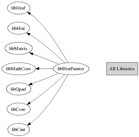
Control routine to paint any kind of histograms.
When you call the Draw method of a histogram for the first time (TH1::Draw),
it creates a THistPainter object and saves a pointer to painter as a
data member of the histogram.
The THistPainter class specializes in the drawing of histograms. It is
separate from the histogram so that one can have histograms without
the graphics overhead, for example in a batch program. The choice
to give each histogram have its own painter rather than a central
singleton painter, allows two histograms to be drawn in two threads
without overwriting the painter's values.
When a displayed histogram is filled again you do not have to call the Draw
method again. The image is refreshed the next time the pad is updated.
A pad is updated after one of these three actions:::Paint
- a carriage control on the ROOT command line
- a click inside the pad
- a call to TPad::Update
By default a call to TH1::Draw clears the pad of all objects before drawing the
new image of the histogram. You can use the "SAME" option to leave the previous
display intact and superimpose the new histogram. The same histogram can be
drawn with different graphics options in different pads.
When a displayed histogram is deleted, its image is automatically removed from the pad.
To create a copy of the histogram when drawing it, you can use TH1::DrawClone. This
will clone the histogram and allow you to change and delete the original one
without affecting the clone.
Setting the Style
Histograms use the current style (gStyle). When you change the current style and
would like to propagate the change to the histogram you can call TH1::UseCurrentStyle.
You will need to call UseCurrentStyle on each histogram.
When reading many histograms from a file and you wish to update them to the current
style you can use gROOT::ForceStyle and all histograms read after this call
will be updated to use the current style.
The following options are supported on all types:
"AXIS" : Draw only axis
"AXIG" : Draw only grid (if the grid is requested)
"HIST" : When an histogram has errors it is visualized by default with
error bars. To visualize it without errors use the option HIST
together with the required option (eg "hist same c").
The "HIST" option can also be used to plot only the histogram
and not the associated function(s).
"FUNC" : When an histogram has a fitted function, this option allows
to draw the fit result only.
"SAME" : Superimpose on previous picture in the same pad
"CYL" : Use Cylindrical coordinates. The X coordinate is mapped on
the angle and the Y coordinate on the cylinder length.
"POL" : Use Polar coordinates. The X coordinate is mapped on the
angle and the Y coordinate on the radius.
"SPH" : Use Spherical coordinates. The X coordinate is mapped on the
latitude and the Y coordinate on the longitude.
"PSR" : Use PseudoRapidity/Phi coordinates. The X coordinate is
mapped on Phi.
"LEGO" : Draw a lego plot with hidden line removal
"LEGO1" : Draw a lego plot with hidden surface removal
"LEGO2" : Draw a lego plot using colors to show the cell contents
When the option "0" is used with any LEGO option, the
empty bins are not drawn.
"SURF" : Draw a surface plot with hidden line removal
"SURF1" : Draw a surface plot with hidden surface removal
"SURF2" : Draw a surface plot using colors to show the cell contents
"SURF3" : same as SURF with in addition a contour view drawn on the top
"SURF4" : Draw a surface using Gouraud shading
"SURF5" : Same as SURF3 but only the colored contour is drawn. Used with
option CYL, SPH or PSR it allows to draw colored contours on a
sphere, a cylinder or a in pseudo rapidy space. In cartesian
or polar coordinates, option SURF3 is used.
"X+" : The X-axis is drawn on the top side of the plot.
"Y+" : The Y-axis is drawn on the right side of the plot.
The following options are supported for 1-D types:
"AH" : Draw histogram without axis. "A" can be combined with any drawing option.
: For instance, "AC" draws the histogram as a smooth Curve without axis.
"][" : When this option is selected the first and last vertical lines
: of the histogram are not drawn.
"B" : Bar chart option
"C" : Draw a smooth Curve througth the histogram bins
"E" : Draw error bars
"E0" : Draw error bars. Markers are drawn for bins with 0 contents
"E1" : Draw error bars with perpendicular lines at the edges
"E2" : Draw error bars with rectangles
"E3" : Draw a fill area througth the end points of the vertical error bars
"E4" : Draw a smoothed filled area through the end points of the error bars
"E5" : Like E3 but ignore the bins with 0 contents
"E6" : Like E4 but ignore the bins with 0 contents
"X0" : When used with one of the "E" option, it suppress the error
bar along X as gStyle->SetErrorX(0) would do.
"L" : Draw a line througth the bin contents
"P" : Draw current marker at each bin except empty bins
"P0" : Draw current marker at each bin including empty bins
"PIE" : Draw a Pie Chart.
"*H" : Draw histogram with a * at each bin
"LF2" : Draw histogram like with option "L" but with a fill area.
: Note that "L" draws also a fill area if the hist fillcolor is set
: but the fill area corresponds to the histogram contour.
"9" : Force histogram to be drawn in high resolution mode.
: By default, the histogram is drawn in low resolution
: in case the number of bins is greater than the number of pixels
: in the current pad.
The following options are supported for 2-D types:
"ARR" : arrow mode. Shows gradient between adjacent cells
"BOX" : a box is drawn for each cell with surface proportional to the
content's absolute value. A negative content is marked with a X.
"BOX1" : a button is drawn for each cell with surface proportional to
content's absolute value. A sunken button is drawn for negative values
a raised one for positive.
"COL" : a box is drawn for each cell with a color scale varying with contents
All the none empty bins are painted. Empty bins are not painted
unless some bins have a negative content because in that case the null
bins might be not empty.
"COLZ" : same as "COL". In addition the color palette is also drawn
"CONT" : Draw a contour plot (same as CONT0)
"CONT0" : Draw a contour plot using surface colors to distinguish contours
"CONT1" : Draw a contour plot using line styles to distinguish contours
"CONT2" : Draw a contour plot using the same line style for all contours
"CONT3" : Draw a contour plot using fill area colors
"CONT4" : Draw a contour plot using surface colors (SURF option at theta = 0)
"CONT5" : (TGraph2D only) Draw a contour plot using Delaunay triangles
"LIST" : Generate a list of TGraph objects for each contour
"FB" : With LEGO or SURFACE, suppress the Front-Box
"BB" : With LEGO or SURFACE, suppress the Back-Box
"A" : With LEGO or SURFACE, suppress the axis
"SCAT" : Draw a scatter-plot (default)
"TEXT" : Draw bin contents as text (format set via gStyle->SetPaintTextFormat)
"TEXTnn" : Draw bin contents as text at angle nn (0 < nn < 90)
"[cutg]" : Draw only the sub-range selected by the TCutG named "cutg"
Most options can be concatenated without spaces or commas, for example:
h->Draw("E1 SAME");
The options are not case sensitive:
h->Draw("e1 same");
The options "BOX", "COL" or "COLZ", use the color palette
defined in the current style (see TStyle::SeTPaletteAxis)
The options "CONT" or "SURF" or "LEGO" have by default 20 equidistant contour
levels, you can change the number of levels with TH1::SetContour or
TStyle::SetNumberContours.
You can also set the default drawing option with TH1::SetOption. To see the current
option use TH1::GetOption.
Setting line, fill, marker, and text attributes
The histogram classes inherit from the attribute classes:
TAttLine, TAttFill, TAttMarker and TAttText.
See the description of these classes for the list of options.
Setting Tick marks on the histogram axis
The TPad::SetTicks method specifies the type of tick marks on the axis.
Assume tx = gPad->GetTickx() and ty = gPad->GetTicky().
tx = 1 ; tick marks on top side are drawn (inside)
tx = 2; tick marks and labels on top side are drawn
ty = 1; tick marks on right side are drawn (inside)
ty = 2; tick marks and labels on right side are drawn
By default only the left Y axis and X bottom axis are drawn (tx = ty = 0)
Use TPad::SetTicks(tx,ty) to set these options
See also The TAxis functions to set specific axis attributes.
In case multiple collor filled histograms are drawn on the same pad, the fill
area may hide the axis tick marks. One can force a redraw of the axis
over all the histograms by calling:
gPad->RedrawAxis();
Giving titles to the X, Y and Z axis
h->GetXaxis()->SetTitle("X axis title");
h->GetYaxis()->SetTitle("Y axis title");
The histogram title and the axis titles can be any TLatex string.
The titles are part of the persistent histogram.
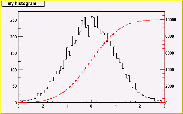
Superimposing two histograms with different scales in the same pad
The following script creates two histograms, the second histogram is
the bins integral of the first one. It shows a procedure to
draw the two histograms in the same pad and it draws the scale of
the second histogram using a new vertical axis on the right side.
(see also tutorial transpad.C for a variant of this example)
void twoscales() {
TCanvas *c1 = new TCanvas("c1","hists with different scales",600,400);
//create/fill draw h1
gStyle->SetOptStat(kFALSE);
TH1F *h1 = new TH1F("h1","my histogram",100,-3,3);
Int_t i;
for (i=0;i<10000;i++) h1->Fill(gRandom->Gaus(0,1));
h1->Draw();
c1->Update();
//create hint1 filled with the bins integral of h1
TH1F *hint1 = new TH1F("hint1","h1 bins integral",100,-3,3);
Float_t sum = 0;
for (i=1;i<=100;i++) {
sum += h1->GetBinContent(i);
hint1->SetBinContent(i,sum);
}
//scale hint1 to the pad coordinates
Float_t rightmax = 1.1*hint1->GetMaximum();
Float_t scale = gPad->GetUymax()/rightmax;
hint1->SetLineColor(kRed);
hint1->Scale(scale);
hint1->Draw("same");
//draw an axis on the right side
TGaxis *axis = new TGaxis(gPad->GetUxmax(),gPad->GetUymin(),
gPad->GetUxmax(), gPad->GetUymax(),0,rightmax,510,"+L");
axis->SetLineColor(kRed);
axis->SetTextColor(kRed);
axis->Draw();
}
/*
*/
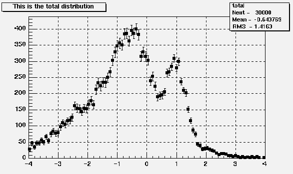
 Statistics Display

 The type of information shown in the histogram statistics box
  can be selected with gStyle->SetOptStat(mode).

  The mode has up to seven digits that can be set to on(1) or off(0).

  mode = iourmen  (default = 0001111)
    n = 1;  name of histogram is printed
    e = 1;  number of entries printed
    m = 1;  mean value printed
    r = 1;  rms printed
    u = 1;  number of underflows printed
    o = 1;  number of overflows printed
    i = 1;  integral of bins printed

 For example: gStyle->SetOptStat(11);
 displays only the name of histogram and the number of entries.
 For example: gStyle->SetOptStat(1101);
 displays the name of histogram, mean value and RMS.
 WARNING: never call SetOptStat(000111); but SetOptStat(1111), 0001111 will
          be taken as an octal number !!
 SetOptStat can also take any combination of letters IOURMEN as its argument.
 For example gStyle->SetOptStat("NE"), gStyle->SetOptStat("NMR") and
 gStyle->SetOptStat("RMEN") are equivalent to the examples above.

 When the histogram is drawn, a TPaveStats object is created and added
 to the list of functions of the histogram. If a TPaveStats object already
 exists in the histogram list of functions, the existing object is just
 updated with the current histogram parameters.
 With the option "same", the statistic box is not redrawn.
 With the option "sames", the statistic box is drawn. If it hiddes
 the previous statistics box, you can change its position
 with these lines (if h is the pointer to the histogram):

  Root > TPaveStats *st = (TPaveStats*)h->FindObject("stats")
  Root > st->SetX1NDC(newx1); //new x start position
  Root > st->SetX2NDC(newx2); //new x end position

 To change the type of information for an histogram with an existing TPaveStats
 you should do: st->SetOptStat(mode) where mode has the same meaning than
 when calling gStyle->SetOptStat(mode) (see above).

 You can delete the stats box for a histogram TH1* h with h->SetStats(0)
 and activate it again with h->SetStats(1).

 Fit Statistics

 You can change the statistics box to display the fit parameters with
 the TStyle::SetOptFit(mode) method. This mode has four digits.
 mode = pcev  (default = 0111)
    v = 1;  print name/values of parameters
    e = 1;  print errors (if e=1, v must be 1)
    c = 1;  print Chisquare/Number of degress of freedom
    p = 1;  print Probability

 For example: gStyle->SetOptFit(1011);
 prints the fit probability, parameter names/values, and errors.


  The ERROR bars options

   'E' default. Shows only the error bars, not a marker
   'E1' Small lines are drawn at the end of the error bars.
   'E2' Error rectangles are drawn.
   'E3' A filled area is drawn through the end points of the vertical error bars.
   '4' A smoothed filled area is drawn through the end points of the
       vertical error bars.
   'E0' Draw also bins with null contents.
/*
*/
  The BAR options

  When the option "bar" or "hbar" is specified, a bar chart is drawn.
   ----Vertical BAR chart: Options "bar","bar0","bar1","bar2","bar3","bar4"
  The bar is filled with the histogram fill color
  The left side of the bar is drawn with a light fill color
  The right side of the bar is drawn with a dark fill color
  The percentage of the bar drawn with either the light or dark color
    is  0 per cent for option "bar" or "bar0"
    is 10 per cent for option "bar1"
    is 20 per cent for option "bar2"
    is 30 per cent for option "bar3"
    is 40 per cent for option "bar4"

  Use TH1::SetBarWidth to control the bar width (default is the bin width)
  Use TH1::SetBarOffset to control the bar offset (default is 0)
    See example in $ROOTSYS/tutorials/hist/hbars.C
/*
*/
   ----Horizontal BAR chart: Options "hbar","hbar0","hbar1","hbar2","hbar3","hbar4"
  An horizontal bar is drawn for each bin.
  The bar is filled with the histogram fill color
  The bottom side of the bar is drawn with a light fill color
  The top side of the bar is drawn with a dark fill color
  The percentage of the bar drawn with either the light or dark color
    is  0 per cent for option "hbar" or "hbar0"
    is 10 per cent for option "hbar1"
    is 20 per cent for option "hbar2"
    is 30 per cent for option "hbar3"
    is 40 per cent for option "hbar4"

  Use TH1::SetBarWidth to control the bar width (default is the bin width)
  Use TH1::SetBarOffset to control the bar offset (default is 0)
    See example in $ROOTSYS/tutorials/hist/hbars.C
/*
*/
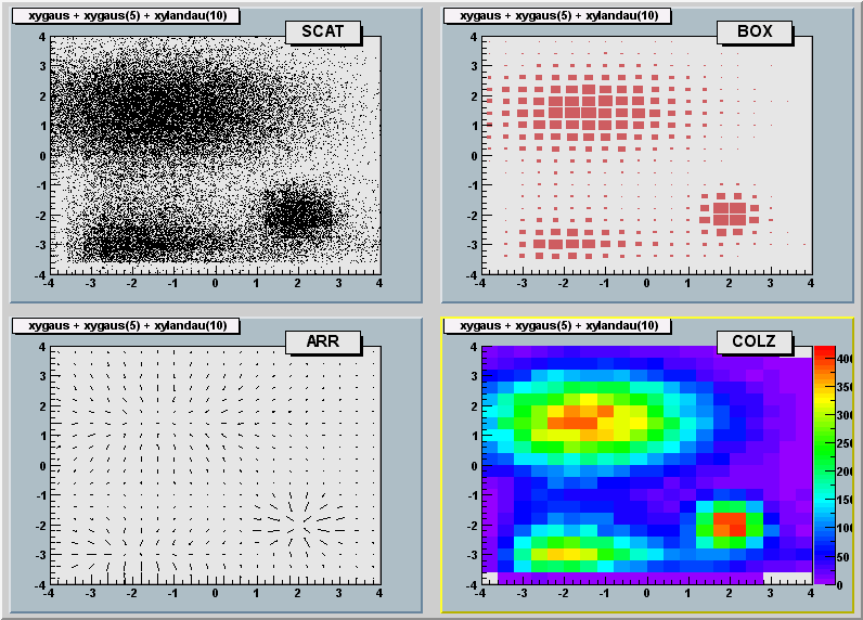
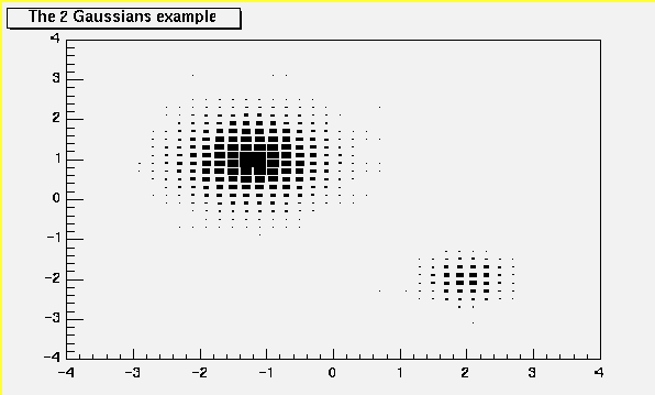
The SCATter plot option (default for 2-D histograms)
For each cell (i,j) a number of points proportional to the cell content is drawn.
A maximum of 500 points per cell are drawn. If the maximum is above 500
contents are normalized to 500.
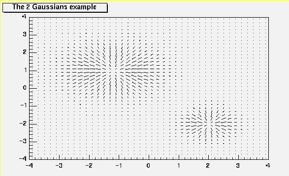
The ARRow option.
Shows gradient between adjacent cells.
For each cell (i,j) an arrow is drawn
The orientation of the arrow follows the cell gradient
The BOX option
For each cell (i,j) a box is drawn with surface proportional to contents
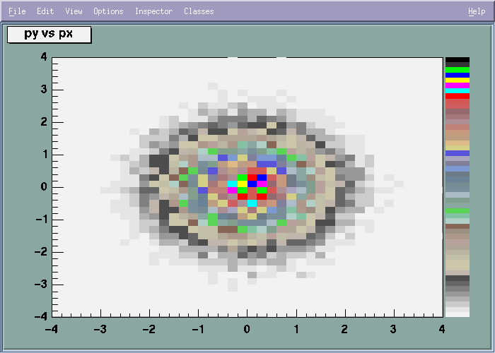
The COLor option
For each cell (i,j) a box is drawn with a color proportional
to the cell content.
The color table used is defined in the current style (gStyle).
The color palette in TStyle can be modified via TStyle::SeTPaletteAxis.
/*
*/
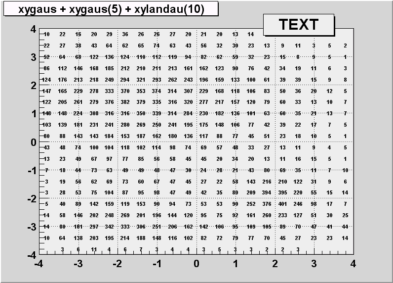
  The TEXT and TEXTnn Option

    For each bin the content is printed.
    The text attributes are:
      - text font = current TStyle font
      - text size = 0.02*padheight*markersize
      - text color= marker color
    "nn" is the angle used to draw the text (0 < nn < 90)
/*
*/
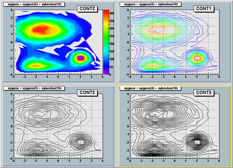
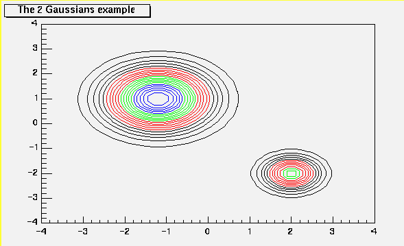
The CONTour options
The following contour options are supported:
"CONT" : Draw a contour plot (same as CONT0)
"CONT0" : Draw a contour plot using surface colors to distinguish contours
"CONT1" : Draw a contour plot using line styles to distinguish contours
"CONT2" : Draw a contour plot using the same line style for all contours
"CONT3" : Draw a contour plot using fill area colors
"CONT4" : Draw a contour plot using surface colors (SURF option at theta = 0)
"CONT5" : Draw a contour plot using Delaunay triangles
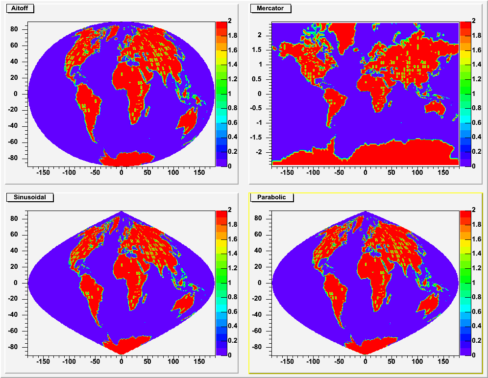
The following options select the "CONT4" option and are usefull for
skymaps or exposure maps. (see example in tutorial earth.C)
"AITOFF" : Draw a contour via an AITOFF projection
"MERCATOR" : Draw a contour via an Mercator projection
"SINUSOIDAL" : Draw a contour via an Sinusoidal projection
"PARABOLIC" : Draw a contour via an Parabolic projection
The default number of contour levels is 20 equidistant levels and can
be changed with TH1::SetContour or TStyle::SetNumberContours.
When option "LIST" is specified together with option "CONT",
the points used to draw the contours are saved in the TGraph object
and are accessible in the following way:
TObjArray *contours =
gROOT->GetListOfSpecials()->FindObject("contours")
Int_t ncontours = contours->GetSize();
TList *list = (TList*)contours->At(i);
Where i is a contour number, and list contains a list of TGraph objects.
For one given contour, more than one disjoint polyline may be generated.
The number of TGraphs per countour is given by list->GetSize().
Here we show only the case to access the first graph in the list.
TGraph *gr1 = (TGraph*)list->First();
/*
*/
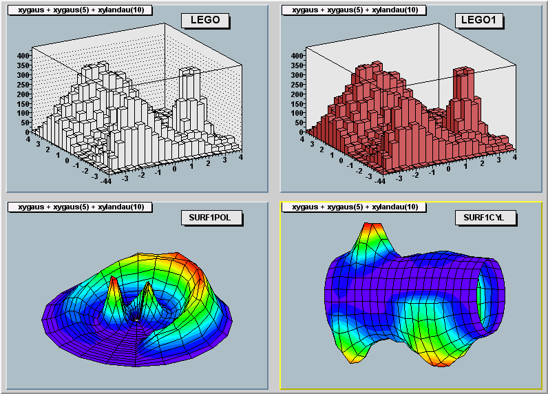
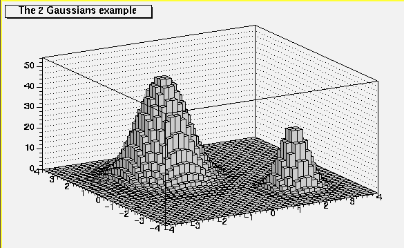
  The LEGO options

    In a lego plot the cell contents are drawn as 3-d boxes, with
    the height of the box proportional to the cell content.
    A lego plot can be represented in several coordinate systems, the
    default system is Cartesian coordinates.
    Other possible coordinate systems are CYL,POL,SPH,PSR.

    "LEGO"   : Draw a lego plot with hidden line removal
    "LEGO1"  : Draw a lego plot with hidden surface removal
    "LEGO2"  : Draw a lego plot using colors to show the cell contents

    When the option "0" is used with any LEGO option, the empty
    bins are not drawn.

    See TStyle::SeTPaletteAxis to change the color palette.
    We suggest you use palette 1 with the call
        gStyle->SetColorPalette(1)
/*
*/
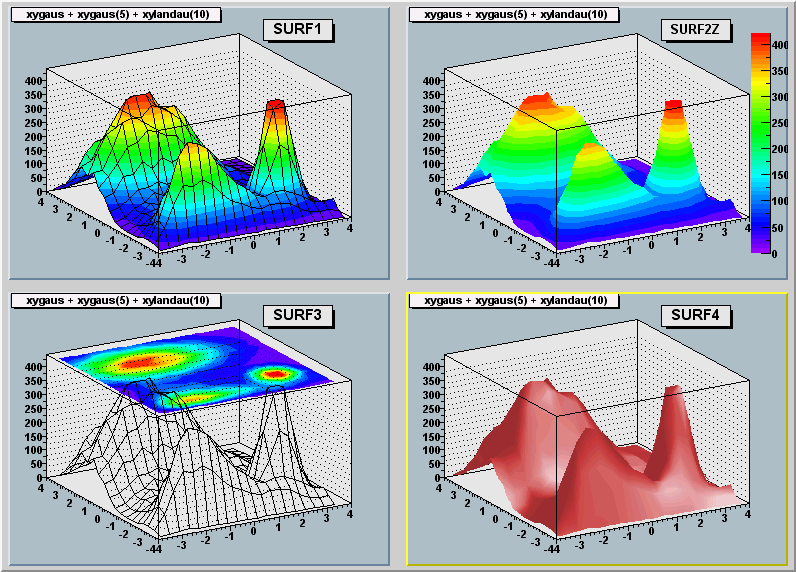
  The "SURFace" options

  In a surface plot, cell contents are represented as a mesh.
     The height of the mesh is proportional to the cell content.

  A surface plot can be represented in several coordinate systems.
  The default is cartesian coordinates, and the other possible systems
  are CYL,POL,SPH,PSR.

    "SURF"   : Draw a surface plot with hidden line removal
    "SURF1"  : Draw a surface plot with hidden surface removal
    "SURF2"  : Draw a surface plot using colors to show the cell contents
    "SURF3"  : same as SURF with in addition a contour view drawn on the top
    "SURF4"  : Draw a surface using Gouraud shading

  The following picture uses SURF1.

      See TStyle::SeTPaletteAxis to change the color palette.
      We suggest you use palette 1 with the call
      gStyle->SetColorPalette(1)
/*
*/
The SPEC option
This option allows to use the TSpectrum2Painter tools. See full
documentation in TSpectrum2Painter::PaintSpectrum.
Option "Z" : Adding the color palette on the right side of the pad
When this option is specified, a color palette with an axis indicating
the value of the corresponding color is drawn on the right side of
the picture. In case, not enough space is left, you can increase the size
of the right margin by calling TPad::SetRightMargin.
The attributes used to display the palette axis values are taken from
the Z axis of the object. For example, you can set the labels size
on the palette axis via hist->GetZaxis()->SetLabelSize().
Setting the color palette
You can set the color palette with TStyle::SeTPaletteAxis, eg
gStyle->SeTPaletteAxis(ncolors,colors);
For example the option "COL" draws a 2-D histogram with cells
represented by a box filled with a color index which is a function
of the cell content.
If the cell content is N, the color index used will be the color number
in colors[N],etc. If the maximum cell content is > ncolors, all
cell contents are scaled to ncolors.
if ncolors <= 0, a default palette (see below) of 50 colors is defined.
This palette is recommended for pads, labels
if ncolors == 1 && colors == 0, a pretty palette with a violet to red
spectrum is created. We recommend you use this palette when drawing legos,
surfaces or contours.
if ncolors > 0 and colors == 0, the default palette is used
with a maximum of ncolors.
The default palette defines:
index 0 to 9 : shades of grey
index 10 to 19 : shades of brown
index 20 to 29 : shades of blue
index 30 to 39 : shades of red
index 40 to 49 : basic colors
The color numbers specified in the palette can be viewed by selecting
the item "colors" in the "VIEW" menu of the canvas toolbar.
The color'a red, green, and blue values can be changed via TColor::SetRGB.
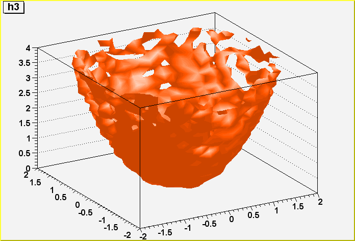
Drawing a sub-range of a 2-D histogram; the [cutg] option
Using a TCutG object, it is possible to draw a sub-range of a 2-D histogram.
One must create a graphical cut (mouse or C++) and specify the name
of the cut between [] in the Draw option.
For example, with a TCutG named "cutg", one can call:
myhist->Draw("surf1 [cutg]");
To invert the cut, it is enough to put a "-" in front of its name:
myhist->Draw("surf1 [-cutg]");
It is possible to apply several cuts ("," means logical AND):
myhist->Draw("surf1 [cutg1,cutg2]");
See a complete example in the tutorial fit2a.C. This example produces
the following picture:
/*
*/
Drawing options for 3-D histograms
By default a 3-d scatter plot is drawn
If option "BOX" is specified, a 3-D box with a volume proportional
to the cell content is drawn.
Drawing using OpenGL
The class TGLHistPainter allows to paint data set using the OpenGL 3D
graphics library. The plotting options start with GL keyword.
General information: plot types and supported options
The following types of plots are provided:
* Lego:
The supported options are:
"GLLEGO" : Draw a lego plot.
"GLLEGO2" : Bins with color levels.
"GLLEGO3" : Cylindrical bars.
Lego painter in cartesian supports logarithmic scales for X, Y, Z.
In polar only Z axis can be logarithmic, in cylindrical only Y.
* Surfaces: (TF2 and TH2 with "GLSURF" options)
The supported options are:
"GLSURF" : Draw a surface.
"GLSURF1" : Surface with color levels
"GLSURF2" : The same as "GLSURF1" but without polygon outlines.
"GLSURF3" : Color level projection on top of plot (works only
in cartesian coordinate system).
"GLSURF4" : Same as "GLSURF" but without polygon outlines.
The surface painting in cartesian coordinates supports logarithmic
scales along X, Y, Z axis.
In polar coordinates only the Z axis can be logarithmic, in cylindrical
coordinates only the Y axis.
Additional options to SURF and LEGO - Coordinate systems:
" " : Default, cartesian coordinates system.
"POL" : Polar coordinates system.
"CYL" : Cylindrical coordinates system.
"SPH" : Spherical coordinates system.
TH3 as boxes (spheres)
The supported options are:
"GLBOX" : TH3 as a set of boxes, size of box is proportional to
bin content.
"GLBOX1": the same as "glbox", but spheres are drawn instead of
boxes.
TH3 as iso-surface(s)
The supported option is:
"GLISO" : TH3 is drawn using iso-surfaces.
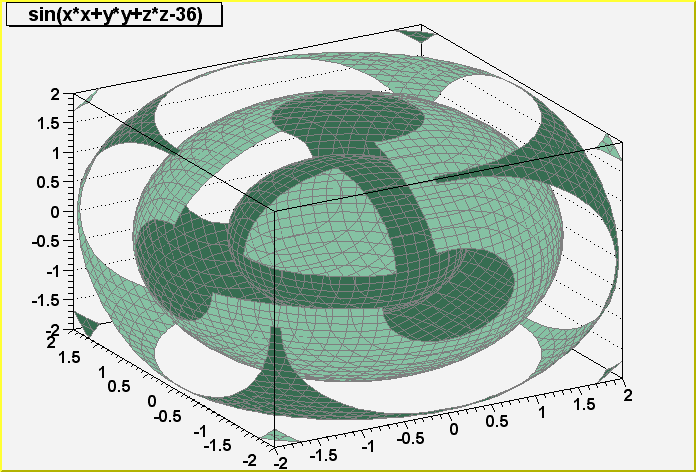
TF3 (implicit function)
The supported option is:
"GLTF3" : Draw a TF3.
Parametric surfaces
$ROOTSYS/tutorials/gl/glparametric.C</tt> shows how to create
parametric equations and visualize the surface.
Interaction with the plots
All the interactions are implemented via standard methods
DistancetoPrimitive and ExecuteEvent. That's why all the interactions
with the OpenGL plots are possible only when the mouse cursor is in the
plot's area (the plot's area is the part of a the pad occupied by
gl-produced picture). If the mouse cursor is not above gl-picture,
the standard pad interaction is performed.
Selectable parts
Different parts of the plot can be selected:
xoz, yoz, xoy back planes:
When such a plane selected, it's highlighted in green if the
dynamic slicing by this plane is supported, and it's
highlighted in red, if the dynamic slicing is not supported.
The plot itself:
On surfaces, the selected surface is outlined in red. (TF3 and
ISO are not outlined). On lego plots, the selected bin is
highlihted. The bin number and content are displayed in pad's
status bar. In box plots, the box or sphere is highlighted and
the bin info is displayed in pad's status bar.
Rotation and zooming
Rotation:
When the plot is selected, it can be rotated by pressing and
holding the left mouse button and move the cursor.
Zoom/Unzoom:
Mouse wheel or 'j', 'J', 'k', 'K' keys.
Panning
The selected plot can be moved in a pad's area by pressing and
holding the left mouse button and the shift key.
Box cut
Surface, iso, box, TF3 and parametric painters support box cut by
pressing the 'c' or 'C' key when the mouse cursor is in a plot's
area. That will display a transparent box, cutting away part of the
surface (or boxes) in order to show internal part of plot. This box
can be moved inside the plot's area (the full size of the box is
equal to the plot's surrounding box) by selecting one of the box
cut axes and pressing the left mouse button to move it.
Plot specific interactions (dynamic slicing etc.)
Currently, all gl-plots support some form of slicing. When back plane
is selected (and if it's highlighted in green) you can press and hold
left mouse button and shift key and move this back plane inside
plot's area, creating the slice. During this "slicing" plot becomes
semi-transparent. To remove all slices (and projected curves for
surfaces) double click with left mouse button in a plot's area.
Surface with option "GLSURF"
The surface profile is displayed on the slicing plane.
The profile projection is drawn on the back plane
by pressing 'p' or 'P' key.
TF3
The contour plot is drawn on the slicing plane. For TF3 the color
scheme can be changed by pressing 's' or 'S'.
Box
The contour plot corresponding to slice plane position is drawn in
real time.
Iso
Slicing is similar to "GLBOX" option.
Parametric plot
No slicing. Additional keys: 's' or 'S' to change color scheme -
about 20 color schemes supported ('s' for "scheme"); 'l' or 'L' to
increase number of polygons ('l' for "level" of details), 'w' or 'W'
to show outlines ('w' for "wireframe").

 */
*/
 */
*/
 */
*/
 */
*/
 */
*/
 */
*/
 */
*/
 */
*/
 */
*/
 */
*/
 */
*/
 */
*/
 */
*/